

Abstract
The magnetic field trapping capability of a bulk superconductor is essentially determined by the critical current density, Jc(B, T), of the material. With state-of-the-art bulk (RE)BCO (where RE = rare earth or Y) materials it is clear that trapped fields of over 20 T are potentially achievable. However, the large Lorentz forces, FL = J × B, that develop during magnetisation of the sample lead to large mechanical stresses that can result in mechanical failure. The radial forces are tensile and the resulting stresses are not resisted well because of the brittle ceramic nature of (RE)BCO materials. Where fields of more than 17 T have been achieved, the samples were reinforced mechanically using resin impregnation and carbon-fibre wrapping or shrink-fit stainless steel. In this paper, two-dimensional (2D) axisymmetric and three-dimensional (3D) finite-element models based on the H-formulation, implemented in the commercial finite element software package COMSOL Multiphysics, are used to provide a comprehensive picture of the mechanical stresses in bulk superconductor magnets with and without mechanical reinforcement during field-cooled magnetisation. The chosen modelling framework couples together electromagnetic, thermal and structural mechanics models, and is extremely flexible in allowing the inclusion of various magnetisation processes and conditions, as well as detailed and realistic properties of the materials involved. The 2D model—a faster route to parametric optimisation—is firstly used to investigate the influence of the ramp rate of the applied field and any heat generated in the bulk. Finally, the 3D model is used to investigate the influence of inhomogeneous Jc(B, T) properties around the ab-plane of the bulk superconductor on the developed mechanical stress.
Export citation and abstract BibTeX RIS

Original content from this work may be used under the terms of the Creative Commons Attribution 3.0 licence. Any further distribution of this work must maintain attribution to the author(s) and the title of the work, journal citation and DOI.
1. Introduction
Bulk superconductors, acting as trapped field magnets, can trap magnetic fields over ten times larger than the maximum fields produced by conventional permanent magnets, which are limited practically to rather less than 2 T [1]. It has been shown that (RE)BCO (where RE = rare earth or Y) bulk superconductors can trap fields greater than 17 T: 17.24 T at 29 K [2] and 17.6 T at 26 K [3] have been demonstrated. The magnetic field trapping capability of a bulk superconductor is essentially determined by the critical current density, Jc(B, T), of the material. With state-of-the-art bulk (RE)BCO materials it is clear that trapped fields of over 20 T are potentially achievable. However, the large Lorentz forces, FL = J × B, that develop during magnetisation of the sample lead to large mechanical stresses that can result in mechanical failure, with unreinforced samples typically failing for magnetic fields greater than 7–9 T [4, 5]. The radial forces are tensile in nature [6] and the resulting stresses are not resisted well because of the brittle ceramic nature of (RE)BCO materials [7]. To achieve the record trapped fields >17 T, the samples were reinforced mechanically using resin impregnation and carbon-fibre wrapping [2] and shrink-fit stainless steel [3].
Extending numerical models developed to date to investigate the magnetisation of bulk superconductors, which have been primarily focused on the electromagnetic and thermal analyses [8], there has been a great deal of interest recently in simulating and analysing the mechanical properties of bulk superconductors using numerical tools [9–14]. These studies have been predominately based on the A-formulation used by Fujishiro et al [9–13], assuming a constant temperature, but the H-formulation was recently used to analyse the stresses developed during pulsed field magnetisation (PFM) by Wu et al [14], which was coupled with a thermal model to include the influence of heat generated during the PFM process.
In this paper, two-dimensional (2D) axisymmetric and three-dimensional (3D) finite-element models based on the H-formulation, implemented in the commercial finite element software package COMSOL Multiphysics [15], are used to provide a comprehensive picture of the mechanical stresses in bulk superconductor magnets with and without mechanical reinforcement during field-cooled magnetisation (FCM). The modelling framework couples electromagnetic, thermal and structural mechanics models, and is extremely flexible to include various magnetisation processes and conditions, as well as detailed and realistic properties of the materials involved. In section 2, the modelling framework is introduced and the results of the 2D and 3D models are compared to demonstrate the consistency of the two models, as well as to show the effect that the reinforcement has on the hoop stress in the bulk during FCM. In section 3, the 2D model—a faster route to parametric optimisation—is firstly used to investigate the influence of varying the ramp rate of the applied field and any heat generated in the bulk. Finally, the 3D model is used to investigate the influence of inhomogeneous Jc(B, T) properties around the ab-plane of the bulk superconductor on the developed mechanical stress.
2. Modelling framework and preliminary results
2.1. Modelling framework
Numerical techniques based on the finite element method (FEM) have been applied to many superconducting material problems using a variety of formulations [8]. Each of these formulations are equivalent in principle, i.e. the choice of formulation should not result in a different physical meaning of the solution, but the solutions of the corresponding partial differential equations can be very different [16]. For more detailed information, including techniques not based on FEM, the reader may refer to recent review papers on numerical methods for calculating AC losses in high-temperature superconducting (HTS) materials [17], the modelling of bulk superconductor magnetisation [8] and HTS applications [18].
A bulk superconductor is usually fabricated in the form of a cylindrical disc and this geometry lends itself well to simplification using a 2D axisymmetric model (r, z, Φ in a cylindrical coordinate system), assuming that its properties are homogeneous in the Φ-direction, i.e. around the bulk's ab-plane. However, a 3D geometry (x, y, z coordinates) is required when including any inhomogeneous material properties around the ab-plane, e.g. differences in Jc between growth sector boundaries (GSBs) and growth sector regions (GSRs) [19], and for shapes without cylindrical symmetry, such as rectangular-shaped bulks [20]. It can also be useful to exploit symmetry, where possible, in a 3D model by applying appropriate boundary conditions to model, for example, one half (2D or 3D) or one quarter of the bulk. This can reduce the number of mesh elements required and improve both computational memory requirements and speed, while retaining the necessary 3D effect. Figure 1(a) shows a 2D axisymmetric model of a disc-shaped bulk superconductor in the r-z-Φ cylindrical coordinate system, making additional use of symmetry along the r-axis to model half the cross-section. The cross-section (Φ-direction; rz-plane) corresponds to the ab-plane of the bulk and the z-axis corresponds to the c-axis. Figure 1(b) shows a 3D model in the x–y–z coordinate system, where geometric symmetry is used to model only 1/8th of the bulk: 1/4 of the bulk around the ab-plane and 1/2 of the bulk along the c-axis (z-axis). In this work, a diameter, D, of 30 mm and thickness, H, of 15 mm are assumed as the dimensions of the bulk, which is a typical size of those fabricated by our research group, and the reinforcement ring is assumed to be 10 mm wide and the same thickness as the bulk.

Figure 1. (a) 2D axisymmetric model of a disc-shaped bulk superconductor with a mechanical reinforcement ring in the r-z-Φ cylindrical coordinate system, making additional use of symmetry along the r-axis to model half the cross-section. (b) 3D model in the x–y–z coordinate system, where geometric symmetry is used to model only 1/8th of the bulk: 1/4 of the bulk around the ab-plane and 1/2 of the bulk along the c-axis (z-axis). In this work, a diameter of 30 mm and thickness of 15 mm are assumed as the dimensions of the bulk, and the reinforcement ring is assumed to be 10 mm wide and the same thickness as the bulk.
Download figure:
Standard image High-resolution imageThe bulk's electromagnetic properties are simulated using the H-formulation, implemented in the commercial software package COMSOL Multiphysics 5.3a [15]. This framework has been used previously by the authors to simulate bulk (RE)BCO materials under various magnetisation conditions [19, 21–26], as well as FCM of MgB2 [27] and iron-pnictide [28] bulks. In the H-formulation, the governing equations are derived from Maxwell's equations—namely, Ampere's (1) and Faraday's (2) laws:


where H = [Hr, Hz] represents the magnetic field components, J = [Jφ] represents the current density and E = [Eφ] represents the electric field in the 2D axisymmetric model. In 3D, H = [Hx, Hy, Hz], J = [Jx, Jy, Jz] and E = [Ex, Ey, Ez]. μ0 is the permeability of free space, and for the superconducting and air sub-domains, the relative permeability can be assumed as simply μr = 1.
The E–J power law [29, 30] is used to simulate the highly non-linear resistivity of the superconductor, where E is proportional to Jn and n = 20 is assumed as a typical value for HTS materials and a good approximation of Bean's critical state model [26].
The results of the numerical simulation depend strongly on the assumed Jc(B, T) characteristics of the material, and in this paper, the measured Jc(B, T) characteristics of a representative bulk HTS (15 wt% Ag-containing GdBa2Cu3O7−δ), presented in [24, 25] for fields up to 10 T over a temperature range of 40–85 K, is extended to 20 T using the equation presented by Jirsa et al in [31]:
Figure 2 shows the assumed Jc(B, T) characteristics, which are input into the model using a two-variable, direct interpolation, as described in [32, 33]. Since FCM is being simulated, there are three distinct steps in the numerical model [27]: (1) applying a ramped external magnetic field parallel to the c-axis of the bulk up to a maximum magnitude, Bapp, by setting appropriate magnetic field boundary conditions [34] such that Hz(t) = Happ(t/tramp) for t ≤ tramp, where Happ = Bapp/μ0 and tramp is the duration of the ramp, while the temperature is held at T > Tc = 92 K (T = 300 K in this paper); (2) cooling the bulk to an appropriate operating temperature, Top ≪ Tc, while the external field is held at Bapp; and (3) once the temperature has stabilised, ramping the external field down from Bapp to zero. Hence, Jc must also be defined for T ≥ Tc = 92 K. Here, Jc is assumed to be 1 × 10⁶ A m−2 for T ≥ 92 K. This is also true for when Jc < 1 × 10⁶ A m−2 for T between 60 K and 85 K in figure 2.

Figure 2. Measured Jc(B, T) characteristics of a representative HTS bulk (15 wt% Ag-containing GdBa2Cu3O7−δ), presented in [24, 25] for fields up to 10 T over a temperature range of 40–85 K, extended here to 20 T using the equation presented by Jirsa et al in [31]. The data is input into the model using a two-variable, direct interpolation, as described in [32, 33].
Download figure:
Standard image High-resolution imageSince the temperature of the bulk changes significantly during FCM, the electromagnetic model is coupled with a thermal model, based on the following thermal transient equation:

The models in this section are coupled through the Jc(B, T) characteristics described earlier and isothermal conditions are assumed while ramping down the field, i.e. Q = 0, because the magnetisation process is slow. It is possible to further couple the electromagnetic and thermal models by including any heat generated during the magnetisation process by assuming Q = Eφ · Jφ (2D axisymmetric model) or Q = Enorm · Jnorm (3D model), where  and
and  This was recently performed in [14] to analyse the stress during PFM and will be used in section 3.1.
Figure 3 shows the time-dependence of the temperature, T(t), as well as the applied magnetic field, Bz(t), during the FCM process as simulated in these models. It should be noted that in section 3.1, the effect of heat generation during ramp down of the field is investigated by including Q = E · J and varying the ramp rate.

Figure 3. Time-dependence of the temperature, T(t), as well as the applied magnetic field, Bz(t), during the FCM process as simulated in these models.
Download figure:
Standard image High-resolution imageFinally, the mechanical stresses during FCM are derived from the following, principal governing equation, an expression of Newton's second law in direct tensor form:

where σs is the Cauchy stress tensor and FL is the Lorentz force (described below). Thus, the structural transient behaviour is assumed to be quasi-static and the second order time-derivatives of the displacement variables, u—the inertial terms, ρd2u/dt2—are zero.
The strain–displacement relationship is given by

where ε is the infinitesimal strain tensor. The bulk is assumed to be an isotropic, linear elastic material, obeying Hooke's law, such that σs = C(E, ν): ε; C is the fourth-order stiffness tensor. Here the mechanical properties of the bulk are defined by its Young's modulus, Ebulk = 1 × 10¹¹ Pa, and Poisson's ratio, νbulk = 0.33 [9–13], and a density, ρbulk = 5900 kg m−3, is assumed [35]. The stainless-steel reinforcement ring, where present, is also assumed to be an isotropic, linear elastic material with Esus = 1.93 × 10¹¹ Pa, νsus = 0.28 and ρsus = 8000 kg m−3 [10–12] and, by default, a perfect mechanical contact between the ring and the bulk is assumed. The Lorentz force, FL = J × B, that develops during the FCM process, derived from the electromagnetic model, is used as the input to calculate the mechanical stresses. Table 1 lists all of the assumed material properties for the coupled electromagnetic-thermal-mechanical modelling, including applicable references to other work in the literature.
Table 1. List of assumed material properties for the coupled electromagnetic-thermal-mechanical modelling of mechanical stresses in bulk superconductor magnets with and without mechanical reinforcement.
| Parameter | Description | Value | Reference(s) (if applicable) |
|---|---|---|---|
| n | n value (E–J power law) | 20 | [8] |
| E0 | Characteristic voltage (E–J power law) | 1 × 10⁻⁴ V m−1 | [8] |
| Jc(B, T) | In-field, temperature-dependent critical current density | Interpolation (see figure 2) | [24, 25] |
| Tc | Superconducting transition temperature (GdBa2Cu3O7−δ) | 92 K | [8] |
| dBup/dt | Ramp rate of applied external magnetic field (ascending stage) | 0.4 T s−1 | |
| dBdown/dt | Ramp rate of applied external magnetic field (descending stage) | 25 mT s−1 | |
| dT/dt | Time rate of change of temperature during cooling (in-field) phase | –1 K s−1 | |
| ρbulk | Density (bulk) | 5900 kg m−3 | [35] |
| ρsus | Density (stainless steel) | 8000 kg m−3 | |
| κab | Thermal conductivity (bulk, ab-plane) | 20 W m−1 K−1 | [8, 35] |
| κc | Thermal conductivity (bulk, c-axis) | 4 W m−1 K−1 | [8, 34] |
| κsus | Thermal conductivity (stainless steel) | Measured data (see ref.) | [24] |
| Cbulk | Heat capacity (bulk) | Measured data (see ref.) | [24] |
| Csus | Heat capacity (stainless steel) | Measured data (see ref.) | [24] |
| αbulk | Coefficient of thermal expansion (bulk) | 5.2 × 10⁻⁶ K−1 | [9–13] |
| αsus | Coefficient of thermal expansion (stainless steel) | 1.27 × 10⁻⁵ K−1 | [10–12] |
| Ebulk | Young's modulus (bulk) | 1 × 10¹¹ Pa | [9–13] |
| Esus | Young's modulus (stainless steel) | 1.93 × 10¹¹ Pa | [10–12] |
| νbulk | Poisson's ratio (bulk) | 0.33 | [9–13] |
| νsus | Poission's ratio (stainless steel) | 0.28 | [10–12] |
2.2. Preliminary results (2D axisymmetric and 3D models)
In this section, the results of the 2D axisymmetric and 3D models are compared, both with and without mechanical reinforcement with a stainless-steel ring, to demonstrate the consistency of the two models, as well as to show the effect that the reinforcement has on the hoop stress in the bulk during FCM.
2.2.1. Without ring reinforcement
Figure 4 shows the trapped field at the centre of the bulk and at the centre of the top surface at z = +0.5 mm above the bulk during the ramp down of the applied field in the FCM process, for the 2D axisymmetric and 3D models, under the following magnetising conditions: Top = 50 K, Bapp = 20 T, dBdown/dt = 25 mT s−1. At the end of the FCM process (t = 1250 s), the trapped field at the centre of the top surface (z = +0.5 mm), Bt, is approximately 7.6 T, and the trapped field at the centre, Bc, is approximately 11.4 T.

Figure 4. Trapped field at the centre of the bulk and at the centre of the top surface at z = +0.5 mm above the bulk during the ramp down of the applied field in the FCM process (t = 1250 s), for the 2D axisymmetric and 3D models, under the following magnetising conditions: Top = 50 K, Bapp = 20 T, dBdown/dt = 25 mT s−1.
Download figure:
Standard image High-resolution imageFigure 5 shows a comparison of the magnetic flux density, ∣B∣, and current density, ∣J∣, distributions throughout the cross-section of the bulk at the end of the FCM process (t = 1250 s), for the 2D axisymmetric and 3D models, under the same magnetising conditions. Figure 6 shows a similar comparison of the Lorentz force in the radial direction, FL,r, and hoop stress, σφ, distributions. The results show clear consistency between the two models and the cross-sectional plots give a clear indication of the location of maximum Lorentz force, as well as maximum hoop stress, which is highest at the centre of the bulk.

Figure 5. Comparison of the magnetic flux density, ∣B∣, and current density, ∣J∣, distributions throughout the cross-section of the bulk at the end of the FCM process (t = 1250 s), for the 2D and 3D models.
Download figure:
Standard image High-resolution image
Figure 6. Comparison of the Lorentz force in the radial direction, FL,r, and hoop stress, σφ, distributions throughout the cross-section of the bulk at the end of the FCM process (t = 1250 s), for the 2D and 3D models.
Download figure:
Standard image High-resolution imageFigure 7 shows the time-dependence of the hoop stress, σφ, across the centre of the bulk (z = 0) at discrete points every 4 T from during the ramp down of the applied field in the FCM process. The results clearly show the dynamic nature of the generated hoop stress, which is directly related to the Lorentz force generated by the distribution of the simultaneously reducing magnetic field, B, and increasing induced current, J, which takes a maximum when the field has ramped down to around 4 T under the given magnetising conditions and material properties. The influence of the reinforcement on the dynamic nature of the hoop stress, as well as its maximum value, is investigated in the next section.

Figure 7. Time-dependence of the hoop stress, σφ, across the centre of the bulk (z = 0 mm) at discrete points every 4 T during the ramp down of the applied field in the FCM process.
Download figure:
Standard image High-resolution image2.2.2. With ring reinforcement
In this section, the same magnetising conditions are assumed (Top = 50 K, Bapp = 20 T, dBdown/dt = 25 mT s−1), but a stainless-steel ring of width 10 mm (inner radius, rinner, of 15 mm, to match the radius of the bulk; outer radius, router, of 25 mm) and the same thickness as the bulk (15 mm) is added around the periphery of the bulk to provide mechanical reinforcement. The resultant plots of the trapped field (see figure 4), as well as ∣B∣ and ∣J∣ (see figure 5) and FL,r (see figure 6) are the same as for the unreinforced case in section 2.2.1; however, the resultant hoop stress changes because of the contribution from the thermal compressive stress applied to the bulk by the reinforcement ring when cooled during FCM (before ramping down the applied field). This occurs due to the difference in the thermal coefficient of expansion between the two materials. A comparison of the hoop stress distributions throughout the cross-sections of the bulk and reinforcement ring at the end of the FCM process (t = 1250 s), for the 2D and 3D models, is shown in figure 8. Again, the results show clear consistency, and it is also clear that the bulk is in compression (negative σφ), whereas the reinforcement ring is in tension (positive σφ), at the end of the FCM process.

Figure 8. Comparison of the hoop stress, σφ, distributions, when including a stainless-steel reinforcement ring that provides a thermal compressive stress when cooled during FCM, for the 2D and 3D models, at the end of the FCM process (t = 1250 s). The same magnetising conditions as section 2.2.1 are assumed: Top = 50 K, Bapp = 20 T, dBdown/dt = 25 mT s−1.
Download figure:
Standard image High-resolution imageFigure 9 shows the time-dependence of the hoop stress, σφ, across the centre of the bulk and reinforcement ring (z = 0) at the beginning (20 T) and end (0 T) of the ramp down of the applied field in the FCM process when the bulk is mechanically reinforced. The results at 4 T, corresponding to the maximum σφ in the unreinforced case (see figure 7), are also shown for comparison. It should be noted that σφ in this case includes both contributions from σφ(FCM), the hoop stress related to the Lorentz force, and σφ(COOL), the thermal compressive stress applied to the bulk by the ring when cooling to Top. The results suggest that for these particular magnetising conditions, there is adequate reinforcement, as the centre of bulk (where the largest hoop stress occurs in the unreinforced case) is in compression, as is the rest of the bulk.

Figure 9. Time-dependence of the hoop stress, σφ, across the centre of the bulk and reinforcement ring (z = 0 mm) at the beginning (20 T) and end (0 T) of the ramp down of the applied field in the FCM process when the bulk is mechanically reinforced. The results at 4 T, corresponding to the maximum σφ in the unreinforced case (see figure 7), are also shown for comparison.
Download figure:
Standard image High-resolution imageFigure 10 shows the time-dependence of the maximum hoop stress, σφ,max, anywhere in the cross-section/volume of the bulk, with and without mechanical reinforcement, as the field is ramped down. For the unreinforced bulk, σφ,max corresponds to the maximum value at the centre of the bulk as shown in figure 7: σφ,max = 63.3 MPa at approximately 4 T. However, for the reinforced bulk, σφ,max (4.9 MPa at approximately 6 T) is not located at the centre of the bulk, but at the edge of the bulk near the surface, which can be seen in figure 8. This was also observed in numerical models for reinforced ring-shaped bulks in [12], and careful optimisation of the ring geometry compared to the bulk is necessary to avoid local stresses and improve the uniformity of the effect of the mechanical reinforcement, which could be carried out easily using this numerical framework.

Figure 10. Time-dependence of the maximum hoop stress, σφ,max, anywhere in the cross-section/volume of the bulk during the ramp down of the applied field in the FCM process, with and without mechanical reinforcement.
Download figure:
Standard image High-resolution image3. Influence of system parameters
The 2D axisymmetric model provides a faster route to parametric optimisation in comparison to the 3D model, if the assumption that the material properties are homogeneous around the bulk's ab-plane holds. In the following sections, the effect of varying the ramp rate of the applied field and any heat generated in the bulk is investigated using the 2D axisymmetric model, and then the 3D model is used to investigate the influence of an inhomogeneous Jc(B) distribution around the bulk's ab-plane.
3.1. Influence of ramp rate and heat generated
3.1.1. Without ring reinforcement
In the simulations so far, isothermal conditions have been assumed, i.e. Q = 0 in equation (4), neglecting the influence of any heat generated during the ramp down of the applied field. In general, the ramp-down rate in the FCM process is usually slow and the heat generated is nowhere near as extreme as that experienced during PFM [14]. However, heat generated during any magnetisation process limits the trapped field capability of the material and it is important to understand how much heat may be generated, as well as its influence on the mechanical stresses in the material. In this section, the heat source, Q = E · J, is introduced to the thermal model (equation (4)), and the influence of three ramp down rates (2.5, 25 and 250 mT s−1) on the FCM process is investigated. It is assumed, as done in section 2.2, that Top = 50 K and Bapp = 20 T.
In the previous analyses, the temperature of the bulk was set by a temperature constraint across the centre of the bulk; however, when including the heat generated during FCM, one must apply a more realistic assumption regarding cooling and here it is assumed that the bulk is cooled from its bottom surface (a typical scenario when magnetised in solenoidal high field magnets), necessitating the removal of the symmetry along the centre of the bulk and modelling of the whole cross-section of the bulk (in the 2D axisymmetric model). It is also possible to cool the sample from the periphery of the bulk for a split coil magnetisation fixture [24]. For simplicity, perfect thermal contact between the bulk and the cryocooler is also assumed; however, as shown in [24, 25, 35], it is possible to adapt the model to include more realistic assumptions regarding this thermal contact, as well as the finite cooling power of the cryocooler.
Figure 11 shows the trapped field at the centre of the top surface at z = +0.5 mm above the bulk during the ramp down of the applied field in the FCM process for ramp-down rates of 2.5, 25 and 250 mT s−1, for Top = 50 K and Bapp = 20 T. As the ramp-down rate is increased, there is a reduction in the trapped field due to a reduction in Jc, which is most noticeable for the fastest ramp rate. Figure 12 shows the temperature of the bulk at the end of the FCM process at t = for 450, 1250 and 8450 s for the three ramp rates, 2.5, 25 and 250 mT s−1, respectively. There is almost no temperature rise for the slowest ramp rate (2.5 mT s−1), and for the intermediate ramp rate (25 mT s−1), there is a temperature rise of around 3 K towards the upper surface of the bulk. In the case of the fastest ramp rate (250 mT s−1), there is a significant temperature rise of up to 18 K in the same region.

Figure 11. Trapped field at the centre of the top surface at z = +0.5 mm above the bulk (without reinforcement) during the ramp down of the applied field in the FCM process for ramp-down rates of 2.5, 25 and 250 mT s−1, for Top = 50 K and Bapp = 20 T. The heat source, Q = E · J, is introduced to include the influence of any heat generated and the bulk is cooled from its bottom surface.
Download figure:
Standard image High-resolution image
Figure 12. Comparison of the temperature distribution within the bulk (without reinforcement) at the end of the FCM process for ramp-down rates of 2.5, 25 and 250 mT s−1, for Top = 50 K and Bapp = 20 T and including the heat source, Q = E · J. The bulk is cooled from its bottom surface.
Download figure:
Standard image High-resolution imageThe impact of this temperature rise on the magnetic flux and current density distributions is shown in figures 13 and 14, respectively, which accounts for the reduced trapped fields in figure 11, except for the 2.5 mT s−1 case. In this case, although the temperature rise is negligible, because the ramp down occurs over a longer time scale (t = 450 → 8450 s), there is more flux creep, resulting in a slightly lower trapped field at the end of the FCM process. The 250 mT s−1 ramp-down rate results in a significantly distorted current density/trapped field distribution, and although there is a small temperature rise for the 25 mT s−1 case, which deviates slightly from the previous assumption of isothermal conditions, a significant impact is not observed.

Figure 13. Comparison of the magnetic flux density, ∣B∣, distribution within the bulk (without reinforcement) at the end of the FCM process for ramp-down rates of 2.5, 25 and 250 mT s−1, for Top = 50 K and Bapp = 20 T and including the heat source, Q = E · J.
Download figure:
Standard image High-resolution image
Figure 14. Comparison of the current density, ∣J∣, distribution within the bulk (without reinforcement) at the end of the FCM process for ramp-down rates of 2.5, 25 and 250 mT s−1, for Top = 50 K and Bapp = 20 T and including the heat source, Q = E · J.
Download figure:
Standard image High-resolution imageThe impact on the developed hoop stress, σφ, within in the bulk is shown in figure 15 at various positions within the bulk, z = 0 and ±6 mm, for the three ramp-down rates, including 25 mT s−1 under the assumption of isothermal conditions. The faster ramp rates, resulting in a higher temperature rise and subsequently reduced Jc, see lower stresses developed overall, which agrees well with the analysis in the previous section. In addition, there is a larger distortion of the stresses between the top and bottom regions of the bulk. In the next section, the impact of the reinforcement ring on these findings is explored.

Figure 15. Hoop stress, σφ, at various positions within the bulk (without reinforcement), z = 0, ±6 mm, at the end of the FCM process for Top = 50 K and Bapp = 20 T and including the heat source, Q = E · J: (a) ramp-down rate of 25 mT s−1 (isothermal conditions), (b) 25 mT s−1, (c) 2.5 mT s−1 and (d) 250 mT s−1.
Download figure:
Standard image High-resolution image3.1.2. With ring reinforcement
The stainless-steel reinforcement ring is now added around the periphery of the bulk and the same magnetising conditions as the previous section are assumed: Top = 50 K, Bapp = 20 T and three ramp-down rates (2.5, 25 and 250 mT s−1), including the heat source, Q = E · J. It is also assumed again that the thermal contact between the bulk, ring and cryocooler is ideal.
Figure 16 shows the trapped field at the centre of the top surface at z = +0.5 mm above the bulk during the ramp down of the applied field in the FCM process for ramp-down rates of 2.5, 25 and 250 mT s−1, for Top = 50 K and Bapp = 20 T. As seen in the previous section, as the ramp-down rate is increased, there is a reduction in the trapped field due to a reduction in Jc, which is most noticeable for the fastest ramp rate. However, there is notably less reduction in trapped field with the reinforcement ring, compared to without one. Figure 17 shows the temperature of the bulk with reinforcement at the end of the FCM process at t = for 450, 1250 and 8450 s for the three ramp rates, 2.5, 25 and 250 mT s−1, respectively. There is almost no temperature rise for the slowest ramp rate (2.5 mT s−1), and for the intermediate ramp rate (25 mT s−1), there is a temperature rise of around 1.2 K towards the upper surface of the bulk (3 K without reinforcement). In the case of the fastest ramp rate (250 mT s−1), the temperature rise is less than 10 K (18 K without reinforcement) in the same region. The presence of the reinforcement ring provides an additional thermal pathway that allows cooling through the ab-plane of the bulk, for which the thermal conductivity is several times larger than along the c-axis [9].

Figure 16. Trapped field at the centre of the top surface at z = +0.5 mm above the bulk (without reinforcement) during the ramp down of the applied field in the FCM process for ramp-down rates of 2.5, 25 and 250 mT s−1, for Top = 50 K and Bapp = 20 T. The heat source, Q = E · J, is introduced to include the influence of any heat generated.
Download figure:
Standard image High-resolution image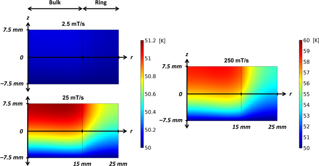
Figure 17. Comparison of the temperature distribution within the bulk (with reinforcement) at the end of the FCM process for ramp-down rates of 2.5, 25 and 250 mT s−1, for Top = 50 K and Bapp = 20 T and including the heat source, Q = E · J.
Download figure:
Standard image High-resolution imageThe impact of the reduced temperature rise on the magnetic flux and current density distributions is shown in figures 18 and 19, respectively, and it is clear that there is less distortion of the current density/trapped field distribution. There is then significantly less distortion of developed hoop stress, σφ, within in the bulk, which is shown in figure 20 at various positions within the bulk, z = 0 and ±6 mm, for the three ramp-down rates, including 25 mT s−1 under the assumption of isothermal conditions. It should be noted again that σφ in this case includes both contributions from σφ(FCM), the hoop stress related to the Lorentz force, and σφ(COOL), the thermal compressive stress applied to the bulk when cooling to Top. There is only a perceptible difference in σφ for the fastest ramp rate (250 mT s−1), meaning that the reinforcement ring not only provides compression of the bulk during the FCM process to avoid mechanical fracture, but provides an additional thermal pathway to remove the heat generated during the magnetisation process, which is particularly useful in the case of PFM.

Figure 18. Comparison of the magnetic flux density, ∣B∣, distribution within the bulk (with reinforcement) at the end of the FCM process for ramp-down rates of 2.5, 25 and 250 mT s−1, for Top = 50 K and Bapp = 20 T and including the heat source, Q = E · J.
Download figure:
Standard image High-resolution image
Figure 19. Comparison of the current density, ∣J∣, distribution within the bulk (with reinforcement) at the end of the FCM process for ramp-down rates of 2.5, 25 and 250 mT s−1, for Top = 50 K and Bapp = 20 T and including the heat source, Q = E · J.
Download figure:
Standard image High-resolution image
Figure 20. Hoop stress, σφ, at various positions within the bulk (with reinforcement), z = 0, ±6 mm, at the end of the FCM process for Top = 50 K and Bapp = 20 T and including the heat source, Q = E · J: (a) ramp-down rate of 25 mT s−1 (isothermal conditions), (b) 25 mT s−1, (c) 2.5 mT s−1 and (d) 250 mT s−1. σφ in this case includes both contributions from σφ(FCM), the hoop stress related to the Lorentz force, and σφ(COOL), the thermal compressive stress applied to the bulk when cooling to Top.
Download figure:
Standard image High-resolution image3.2. Inhomogeneous Jc distribution around the ab-plane
Although the 2D axisymmetric model provides a faster route to parametric optimisation, this assumes that the material properties are homogeneous around the bulk's ab-plane. In this section, the 3D model is used to investigate an example of the influence of inhomogeneous material properties around the ab-plane, such as those that occur during the growth process of c-axis seeded, single grain (RE)BCO bulk superconductors [19]. The 3D model is also useful for shapes without cylindrical symmetry, such as rectangular-shaped bulks [20].
Following the same method presented in [19, 36], the Jc(B, T) characteristics are varied using a cosine function around the ab-plane, supposing some difference of ±10% in Jc between the GSBs and GSRs, such that

Given the relevant material properties are known, by measuring a number of sub-specimens from a bulk superconductor, any position-dependent Jc could be introduced in the model.
The same magnetising conditions as the previous sections are assumed: Top = 50 K, Bapp = 20 T and a ramp-down rate of 25 mT s−1 under isothermal conditions (Q = 0). At the end of the FCM process (t = 1250 s), the trapped field at the centre of the top surface (z = +0.5 mm), Bt, of the inhomogeneous bulk is approximately 7.4 T, and the trapped field at the centre, Bc, is approximately 11 T (see 7.6 T and 11.4 T, respectively, for the homogeneous bulk described in section 2.2.1).
Figure 21 shows a 3D picture of the hoop stress, σφ, distributions for the homogeneous (left) and inhomogeneous (right) Jc assumptions at the end of the FCM process and figure 22 shows a 2D surface plot of σφ across the centre of the bulk (xy-plane, where the c-axis is oriented along the z-axis), where the supposed GSBs and GSRs are highlighted by dotted and dashed white lines, respectively. It is clear that the inhomogeneous ab-plane Jc distorts σφ with lower stress in low-Jc regions and higher stress in high-Jc regions. Figure 23 shows a 2D plot of the σφ distributions for the homogeneous and inhomogeneous Jc assumptions at z = 0 mm, i.e. across the centre of the bulk. The plots for the inhomogeneous bulk correspond to the supposed GSBs and GSRs highlighted in figure 22. This further emphasises the difference between the stresses developed in an inhomogeneous bulk compared to a homogeneous one and shows how the 3D model is useful for incorporating more realistic assumptions when a 2D axisymmetric model is insufficient.

Figure 21. 3D volume plot of the hoop stress, σφ, distributions of an unreinforced bulk superconductor at the end of the FCM process, assuming homogeneous Jc properties around the ab-plane (left) and inhomogeneous properties (right) supposing some difference of ±10% in Jc between the growth sector boundaries (GSBs) and growth sector regions (GSRs).
Download figure:
Standard image High-resolution image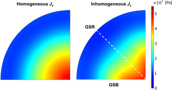
Figure 22. 2D surface plot, cut across the centre of the bulk (xy-plane), of the hoop stress, σφ, distributions of an unreinforced bulk superconductor at the end of the FCM process for the homogeneous (left) and inhomogeneous (right) Jc assumptions. The supposed GSBs and GSRs are highlighted by dotted and dashed white lines, respectively.
Download figure:
Standard image High-resolution image
Figure 23. 2D plot of the hoop stress, σφ, distributions of an unreinforced bulk superconductor at the end of the FCM process for the homogeneous and inhomogeneous Jc assumptions at z = 0 mm. The plots for the inhomogeneous bulk correspond to the supposed GSBs and GSRs highlighted in figure 22.
Download figure:
Standard image High-resolution imageFigure 24 shows the 2D surface plot of σφ across the centre of the bulk (xy-plane) and figure 25 shows a 2D plot of σφ across the centre of the bulk at z = 0 mm along the supposed GSBs and GSRs at the end of the FCM process, in the case that the bulk is reinforced by the stainless-steel ring. In order to better highlight the differences within the homogeneous and inhomogeneous bulks, the ring is not included in these plots. Here σφ includes both contributions from σφ(FCM), the hoop stress related to the Lorentz force, and σφ(COOL), the thermal compressive stress applied to the bulk when cooling to Top. The trends for σφ are identical to those shown in figures 22 and 23 for the unreinforced case; however, there is an offset owing to σφ(COOL), such that σφ is entirely negative (and less than 60 MPa). Thus, the 3D model provides a useful tool to analyse the influence of inhomogeneous material properties and design adequate reinforcement so that mechanical fracture is avoided in high magnetic fields.
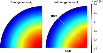
Figure 24. 2D surface plot, cut across the centre of the bulk (xy-plane), of the hoop stress, σφ, distributions of a reinforced bulk superconductor (ring not shown) at the end of the FCM process for the homogeneous (left) and inhomogeneous (right) Jc assumptions. The supposed GSBs and GSRs are highlighted by dotted and dashed white lines, respectively.
Download figure:
Standard image High-resolution image
Figure 25. 2D plot of the hoop stress, σφ, distributions of a reinforced bulk superconductor at the end of the FCM process for the homogeneous and inhomogeneous Jc assumptions at z = 0 mm. The plots for the inhomogeneous bulk correspond to the supposed GSBs and GSRs highlighted in figure 24.
Download figure:
Standard image High-resolution image
4. Conclusion
In this paper, 2D axisymmetric and 3D finite-element models based on the H-formulation, implemented in the commercial finite element software package COMSOL Multiphysics, are used to analyse the mechanical stresses in bulk superconductor magnets during FCM with and without mechanical reinforcement using a stainless-steel ring.
- 1.Under identical magnetising conditions and assuming the same material properties, the 2D axisymmetric and 3D finite-element models produce consistent results: the 2D model provides a faster route to parametric optimisation, but the 3D model is required for bulk superconductor shapes that do not have cylindrical symmetry or for inhomogeneous properties in the Φ-direction, i.e. around the ab-plane. The models can be used to examine the stresses developed during the magnetisation process, which depend on a number of important factors, including the Jc(B, T) characteristics, sample geometry, ramp-down rate and so on. It is shown how the use of a mechanical reinforcement ring, with a higher coefficient of thermal expansion than the bulk superconductor, significantly reduces the mechanical stresses developed during FCM owing to σφ(COOL), the thermal compressive stress applied to the bulk by the ring when cooling to the operating temperature, Top.
- 2.The 2D axisymmetric model, assuming homogeneous properties around the ab-plane, is used as a fast optimisation tool to investigate the influence of any heat generated during the ramp down of the applied field by including the heat source, Q = E · J. A faster ramp-down rate of the applied field results in a larger temperature rise, resulting in an uneven temperature distribution within the bulk, depending on the method of cooling. This will distort the magnetic flux and current density distributions, which, in turn, affect the developed stresses. The presence of a reinforcement ring not only provides compression of the bulk during FCM to avoid mechanical fracture, but also provides an additional thermal pathway to remove the heat generated during the magnetisation process, which is particularly useful to consider in the case of PFM.
- 3.The 3D model is used to investigate the influence of inhomogeneous Jc(B, T) properties around the ab-plane and it shown how the developed hoop stress is distorted, with lower stress in low-Jc regions and higher stress in high-Jc regions. When the bulk is reinforced with a stainless-steel ring, the trends for σφ are identical to those in the unreinforced case; however, there is an offset owing to σφ(COOL), such that σφ is entirely negative under the conditions analysed.
The modelling framework couples together electromagnetic, thermal and structural mechanics models to provide a complete and detailed picture of the mechanical stresses developed in a bulk superconductor during the FCM process and a useful and flexible design tool to adequately reinforce the bulk to avoid mechanical fracture at high magnetic fields, taking into account many of the practical situations faced when carrying out such high field experiments.
Acknowledgments
Dr Mark Ainslie would like to acknowledge financial support from an Engineering and Physical Sciences Research Council (EPSRC) Early Career Fellowship EP/P020313/1. All data are provided in full in the results section of this paper. Mr Kaiyuan Huang would like to acknowledge financial support from Siemens AG, Corporate Technology, Munich, Germany. Professor Hiroyuki Fujishiro would like to acknowledge financial support from JSPS KAKENHI Grant No. JP15K04646.
Appendix
Some comments on the implementation in COMSOL Multiphysics of the modelling framework described in section 2.2 are provided as follows.
- 1.The electromagnetic model is implemented using the 'Magnetic Field Formulation' interface in COMSOL's AC/DC module.
- 2.In order to make use of the symmetry in the 3D model (see figure 1(b)), additional boundary conditions must also be set for the sides (yz-plane, x = 0; xz-plane, y = 0) and bottom plane of the entire geometry: (xy-plane, z = 0): this is achieved using the 'Magnetic Insulation' node for the former (setting the tangential component of the magnetic potential to zero) and the 'Perfect Magnetic Conductor' node for the latter (setting the tangential component of the magnetic field to zero).
- 3.The thermal model is implemented using COMSOL's 'Heat Transfer in Solids' interface and the temperature, T(t), is set by applying a constraint across the centre of the bulk in the z = 0 plane.
- 4.The electromagnetic and thermal models are coupled with COMSOL's 'Solid Mechanics' interface in its Structural Mechanics module to include analyses of the mechanical stresses during FCM. A 'roller' constraint (equivalent to a symmetry condition) is applied to the bulk (and ring when applicable) in the z = 0 plane, making the displacement in the direction normal to this plane zero.
- 5.The Lorentz force, FL = J × B, is implemented as a force per unit volume using the 'Body Load' node where Fr = Bz · Jφ and Fz = –Br · Jφ (2D axisymmetric model) or Fx = Jy · Bz – Jz · By, Fy = Jz · Bx – Jx · Bz and Fz = Jx · By – JyBx (3D model).
- 6.A thermal coefficient of expansion is included for both the bulk and reinforcement ring (see table 1) using COMSOL's 'Thermal Expansion' multiphysics interface to simulate the thermal compressive stress applied to the bulk by the reinforcement ring when cooled during FCM because of the difference in this coefficient between the two materials [9].