
Abstract
Static and dynamic polarizabilities are calculated for the non-relativistic hydrogen molecular ion by solving the three-body Schrödinger equation in perimetric coordinates with the Lagrange-mesh method. The static dipole polarizabilities of the ground-state rotational band are computed for total orbital (or rotational) angular momenta from L = 0 to 39 with an absolute accuracy of about 10−9 au. For L = 0, 1 and 2, slightly less accurate results are also given for the first three vibrational excited levels. For the ground state, dynamic dipole polarizabilities as well as static and dynamic quadrupole polarizabilities are computed. To illustrate the versatility of the method, the static dipole polarizability of the hydrogen molecular ion in a Debye plasma is also determined.
Export citation and abstract BibTeX RIS
1. Introduction
The hydrogen molecular ion H+2 is the most fundamental molecular system that exists in nature. It is thus important to calculate its properties as accurately as possible and to verify whether they agree with experiment, when possible. An interesting observable is the electric dipole polarizability. Dipole polarizabilities have been measured for the ground state [1–3] and the first rotational excited level [4] of H+2 in a series of experiments on the Rydberg states of H2. Some disagreement was observed between the first experimental results for the ground state [1, 2] and calculations at the Born–Oppenheimer approximation [5] and some of its improvements. This encouraged fully quantal calculations solving the three-body Schrödinger equation as accurately as possible. Different methods have been applied to consider the non-adiabatic study of the ground-state polarizability of this system [6–10]. These calculations reconciled theory with experiment. A similar evolution occurred for the first excited rotational level where elaborate theory [11, 12] agrees with experiment [4]. However, an improved measurement of the ground-state polarizability [3] again led to a disagreement with theory. Further, more accurate theoretical works do not solve this discrepancy [13–15].
In this work, we consider the three-body Schrödinger equation with only Coulomb forces in the Hamiltonian, i.e. without electron and nuclear spin effects. In this case, the Hamiltonian is invariant under purely spatial rotations and under reflection, with respect to the centre of mass of the molecular ion. Hence, the total orbital angular momentum L and the parity π are good quantum numbers [16–18]. The total intrinsic spin of the three particles does not play a role, but the total spin of the protons is related to the symmetry of the spatial part of the wavefunctions [19]. The present notation and terminology is based on the good quantum numbers of a three-body problem and may differ from the ones used in molecular physics where L is called the total rotational angular momentum which is sometimes denoted as J. The notation L used here emphasizes that the electron and proton spins are not included in its definition. For each Lπ value, several excited states can be obtained when solving the three-body Schrödinger equation. The excited levels correspond to vibrational excitations in the Born–Oppenheimer framework. For this reason, we denote the excitation quantum number as v, with v = 0 for the lowest state. A given level is thus fully defined by (Lπ, v). A set of levels with the same value of v form a rotational band. We limit this study to bound states corresponding to the Σg electronic configuration. Because of the identity of the protons, even-L states then correspond to a total intrinsic spin 1/2 for the molecule (the total spin of the protons is 0), while odd-L states correspond to a total spin 1/2 or 3/2 (the total spin of the protons is 1) [19].
In the non-adiabatic approximation, the spectrum of H+2 has been obtained with high precision using different approaches (see [19] and references therein). It is interesting to try to reach a similar accuracy for other observables, and in particular for the polarizabilities [11–15]. The most accurate result for the ground state has been obtained by Yan et al [15]. Dipole polarizabilities for vibrational levels from v = 0 to 10 were accurately calculated by Hilico et al [14] and the first excited rotational level was studied by Moss in a fully nonadiabatic way [11, 12]. Korobov studied the importance of relativistic corrections for the ground state [13].
Recently, we have accurately calculated not only energies and wavefunctions of the four lowest vibrational bound or quasi-bound levels (v = 0 to 3) for total orbital momenta from L = 0 to 40, but also all possible transition probabilities between these levels [19]. These transitions are quadrupolar since dipole transitions are forbidden within the Σg band. Using wavefunctions from our previous work [19], we now present accurate dipole polarizabilities for the whole ground-state rotational band of the molecular ion H+2. They are obtained from three-body wavefunctions calculated in perimetric coordinates [20, 21] with the Lagrange-mesh method [16–18]. This method has proved to be particularly simple and very precise for the determination of static and dynamic polarizabilities in the case of the confined hydrogen atom [22]. Dynamic polarizabilities of the ground state as well as quadrupole polarizabilities of the four lowest L = 0 levels are considered. We show that the method also applies to H+2 in a Debye plasma.
The Lagrange-mesh method is an approximate variational calculation using a basis of Lagrange functions, i.e. functions that vanish at all points but one of a three-dimensional mesh, and the Gauss quadrature associated with this mesh [23, 24]. The accuracy of the lowest energies exceeds by far the accuracy of the Gauss quadrature for the individual matrix elements [25]. The exponential convergence of the Lagrange-mesh method is typical of pseudo-spectral methods. With the analytical approximations to the wavefunctions provided by the Lagrange-mesh method, the matrix elements in the calculation of the dipole and quadrupole polarizabilities are simple expressions when used with the corresponding Gauss–Laguerre quadrature.
In section 2, the definition of the dynamic multipole polarizabilities is presented. The expansion of the rotational–vibrational wavefunctions in perimetric coordinates together with the Lagrange-mesh technique is summarized. In section 3, static and dynamic dipole and quadrupole polarizabilities for the molecular ion H+2 are given and discussed. The application of the method to the molecular ion immersed in a hot Debye plasma [26] is also illustrated. Concluding remarks are presented in section 4. Atomic units are used throughout.
2. Lagrange-mesh calculation of transition probabilities
2.1. Dynamic electric polarizability
A system of charged particles described by a Hamiltonian H is in a state of energy E with wavefunction Ψ. It is perturbed by an electric multipole O(λ)μ of multipolarity λ and projection μ oscillating at angular frequency ω,

Following the perturbation theory presented in [27] and [28], the equation of the first-order correction Ψ( ± ) to the wavefunction Ψ is

The frequency-dependent multipole polarizability αλμ(ω) for the state Ψ is given by

For the H+2 molecular ion, the three-body Hamiltonian involving the Coulomb interactions between the three particles but no spin effects reads

where 1 and 2 refer to the proton coordinates, mp is the proton mass and e refers to the electron coordinate. It depends upon the interproton distance R and the two distances re1 and re2 between the electron and the protons. Its eigenfunctions  depend on the total orbital (or rotational) angular momentum L, its projection M, the parity π and the spatial symmetry σ of the protons. The total spin of the protons is fixed by σ = ( − 1)S. The many bound states corresponding to the Σg electronic configuration have π = σ = ( − 1)L and the three weakly bound levels corresponding to the Σu electronic configuration have π = −σ = ( − 1)L. The corresponding energies are denoted as
  . For simplicity, we shall drop the σ superscript in the following as the electric transition operators conserve the spatial proton symmetry. The polarizabilities are calculated below for the levels of the Σg electronic configuration.
2.2. Expansions of the wavefunctions
We approximatively solve the Schrödinger equation for the hydrogen molecular ion H+2 without using the Born–Oppenheimer approximation and its corrections. To this end, the Lagrange-mesh method [23–25] in perimetric coordinates [20, 21] is used as explained in [18, 19].
The perimetric system of coordinates involves the three Euler angles ψ, θ and ϕ which characterize the orientation of the molecular plane and the three combinations of interdistances:

The wavefunctions are expanded over a basis of angular functions as [18]

The internal degrees of freedom are described by ΦLπK(x, y, z) in terms of the perimetric coordinates. The normalized angular functions  are defined for K ⩾ 0 by
where DLMK(ψ, θ, ϕ) represents a Wigner matrix element. They have parity π and change as π( − 1)K under permutation of the protons. Hence, ΦLπK is symmetric for ( − 1)K = σπ and antisymmetric for ( − 1)K = −σπ, when x and y are exchanged. When (6) is introduced in the Schrödinger equation, one obtains the system of coupled equations

where  are the matrix elements of the Hamiltonian evaluated between angular functions [17, 18].
The electric transition operators can be written in perimetric coordinates as [19]

The perimetric coefficients  are given in terms of the interprotonic distance R and the polar components of the electron coordinate (ρ, ζ) for the dipole (λ = 1) as

with the total mass M = 2mp + 1 and for the quadrupole (λ = 2) as
with γ = 1 − 2M−1 − M−2. See [18, 19] for the expressions of R, ρ and ζ in terms of the perimetric coordinates.
Now, one needs to solve equations (2). Their solutions depend on both M and μ for each Lπσ. For this purpose, we expand the  functions as

where  also depends on Lπ but this dependence is understood. The Clebsch–Gordan coefficients are introduced for later convenience. After the substitution of the functions
  and
and  in equation (2), the dependence on M and μ disappears and one obtains the system of differential equations:

The coefficients  are given by

See the definition in [19] where a factor (LλMμ|L'M') is missing on the left-hand side of equation (21).
2.3. Lagrange-mesh method
In order to solve the system (13), we apply the Lagrange-mesh method [23, 18] which is an approximatively variational calculation with Lagrange basis functions FKijk(x, y, z) [18, 19]. The Lagrange functions have the remarkable property that they vanish at all mesh points (hxui, hyvj, hzwk) of an associated mesh, but one. The ui, vj and wk are the zeros of Lagrange polynomials of respective degrees Nx, Ny and Nz and, hx, hy and hz are scaling factors. The variational calculation is simplified by the use of a Gauss quadrature associated with the mesh. In this method, the ΦK(x, y, z) functions of equation (6) are expanded as [18]
where we use the same number N of mesh points and the same scale factor h for the two perimetric coordinates x and y. Because of the symmetrization, the sum over j is limited by the value i − δK, where δK is equal to 0 when ( − 1)K = σπ and to 1 when ( − 1)K = −σπ. A similar expansion is used for Φ( ± )LπK(x, y, z) with coefficients C( ± )LπKijk.
With the Gauss quadrature, equations (8) become a linear system for the coefficients CLπKijk [18],
The eigenvalues of the Hamiltonian matrix are denoted as  , where v is the level of vibrational excitation. The corresponding wavefunctions are available analytically when the coefficients CLπKijk are introduced in (15) and (6). In our previous work [19], the spectra of the four lowest vibrational, v = 0 to 3, and 41 rotational states, L = 0 to 40, were obtained as well as analytic approximations for the corresponding wavefunctions that are employed here.
A similar treatment of the differential system (13) leads to the inhomogeneous algebraic system of equations:

The coefficients  are for the dipole transition operator (λ = 1):

and for the quadrupole transitions operator (λ = 2):

2.4. Polarizabilities
With the expansions of the wavefunction  and of the first order correction
  due to an electric perturbation of the hydrogen molecular ion, the polarizability (3) can be directly calculated as

where

The perimetric matrix elements  are calculated from (10) and (11) by integration over the perimetric coordinates with the volume element (x + y)(y + z)(z + x) dx dy dz. In practice, the sums over K and K' are truncated at Kmax. The α(LM)λμ components satisfy the symmetry relations α(L − M)λ − μ = αλμ(LM).
The remaining calculation of the matrix elements is particularly simple within the Lagrange-mesh method. Because the Lagrange functions vanish at all mesh points but one, the matrix elements in (21) are simply obtained with the Gauss quadrature as

where  .
.
Due to the orthogonality relations of the Clebsch–Gordan coefficients, the polarizabilities averaged over M,

do not depend on μ and can be easily calculated with

Then, any μ-component of the polarizability (20) and the average polarizability (23) can be obtained from the 2λ + 1 coefficients  .
.
3. Polarizability
3.1. Static electric dipole polarizabilities
After solving the linear system (17) for the coefficients C( ± )LπKijk, the approximation to the first correction  are obtained. For convenience, we use the same wavefunctions ΨLπM for the free hydrogen molecular ion as in [19]. The same numbers of mesh points are employed: N = Nx = Ny = 40 for the x and y coordinates and Nz = 20 for the z coordinate. The scale parameters are h = hx = hy = 0.14 and hz = 0.4. For a given K value, the total number of basis states is then 16 400 or 15 600 depending on the parity of K. The size of the sparse Hamiltonian matrix is larger by about a factor (Kmax + 1) when K is limited by K ⩽ Kmax ⩽ L. For L > 2, like in [18], calculations are performed with Kmax = 2. The conventional value for the proton mass: mp = 1836.152701 au is used.
Table 1 shows a convergence test of the energies and static polarizabilities of the first four vibrational levels v = 0 to 3 for L = 0 as a function of the numbers of mesh points. The nonlinear scale parameters are hx = hy = 0.14 and hz = 0.4. The results of table 1 show that the convergence with Nz is reached faster than with N, i.e. already with Nz = 20. For the slower N convergence, one observes that adding five points leads to an exponential improvement by a factor of about 30 for both energies and polarizabilities. By extrapolation, the absolute accuracy of the dipole polarizability α(0)1 with (40, 20) is about 10−10 for the (0+, 0) state and decreases to 10−8 for (0+, 1), 10−7 for (0+, 2) and 10−6 for (0+, 3). We have checked for L = 0 and L = 30 that the v = 0 polarizabilities do not change by more than 2 × 10⁻⁹ when hx = hy vary from 0.12 to 0.16 and hz varies from 0.35 to 0.60. Note that the Hamiltonian matrices completely change when the scale parameters are modified. The chosen values, where the accuracy is optimal over the whole rotational bands, lie within this stability plateau.
Table 1. Convergence of the energies E0 +v and dipole polarizabilities α(0)1, v as a function of the numbers of mesh points N and Nz for the ground state (0+, 0) and the three lowest vibrational levels (0+, 1), (0+, 2) and (0+, 3). The most accurate theoretical and experimental results are also presented.
| N | Nz |  |
α(0)1, 0 |  |
α(0)1, 1 |
|---|---|---|---|---|---|
| 20 | 20 | −0.597 138 545 | 3.168 934 | −0.587 144 6 | 3.9035 |
| 25 | 20 | −0.597 139 051 2 | 3.168 732 36 | −0.587 155 355 | 3.897 787 |
| 30 | 20 | −0.597 139 062 838 | 3.168 725 999 | −0.587 155 670 45 | 3.897 569 78 |
| 35 | 20 | −0.597 139 063 116 8 | 3.168 725 807 04 | −0.587 155 679 003 | 3.897 563 54 |
| 40 | 20 | −0.597 139 063 123 2 | 3.168 725 802 80 | −0.587 155 679 206 | 3.897 563 36 |
| 35 | 30 | −0.597 139 063 116 8 | 3.168 725 807 03 | −0.587 155 679 003 | 3.897 563 54 |
| 40 | 30 | −0.597 139 063 123 2 | 3.168 725 802 79 | −0.587 155 679 206 | 3.897 563 36 |
| 50 | 25 | −0.597 139 063 123 4 | 3.168 725 802 65 | −0.587 155 679 212 | 3.897 563 35 |
| [9] | 3.168 7256 | ||||
| [10] | 3.168 726 | ||||
| [14] | 3.168 725 803 | 3.897 563 360 | |||
| [15] | 3.168 725 802 67 | ||||
| [3] (exp.) | 3.167 96(15) | ||||
| N | Nz |  |
α(0)1, 2 |  |
α(0)1, 3 |
| 20 | 20 | −0.577 660 | 4.8621 | −0.568 50 | 6.27 |
| 25 | 20 | −0.577 748 20 | 4.824 013 | −0.568 884 | 6.030 |
| 30 | 20 | −0.577 751 788 | 4.821 5997 | −0.568 907 47 | 6.010 59 |
| 35 | 20 | −0.577 751 901 0 | 4.821 504 47 | −0.568 908 459 | 6.009 379 |
| 40 | 20 | −0.577 751 904 4 | 4.821 500 47 | −0.568 908 497 | 6.009 329 |
| 35 | 30 | −0.577 751 901 0 | 4.821 504 47 | −0.568 908 459 | 6.009 379 |
| 40 | 30 | −0.577 751 904 4 | 4.821 500 47 | −0.568 908 497 | 6.009 329 |
| 50 | 25 | −0.577 751 904 5 | 4.821 500 36 | −0.568 908 498 | 6.009 327 |
| [14] | 4.821 500 365 | 6.009 327 479 |
The accuracy of the present matrix elements as well as the accuracies of other observables in [18] and of the transition probabilities in [19] indicate that the present wavefunctions have relative accuracies better than 10−7 for v = 0 to 2 over most of the various rotational bands and are a little less good for v = 3.
A comparison with the best theoretical results is also presented in table 1. The results of Yan et al [15] for the ground state and of Hilico et al [14] for the vibrationally excited states are more accurate than ours. When the number of mesh points are increased to N = 50, Nz = 25 our results are in agreement with those presented by Hilico et al [14]. The ground-state polarizability has been investigated in several papers [9, 10, 13–15] and all of them are in agreement in at least seven significant digits. However, a difference with the experimental result [3] arises at the fifth significant digit. Relativistic corrections only slightly reduce the problem [13]. The origin of this disagreement remains unclear but does not arise from inaccuracies in the numerical resolution of the three-body Schrödinger equation.
Table 2 presents an extensive list of the components α(LL − 1)1, α(LL)1 and α(LL + 1)1 of the dipole polarizabilities for the full rotational band (L = 0 to 39) corresponding to the lowest vibrational level v = 0. According to (20), any M-component can be calculated with multiplications by Clebsch–Gordan coefficients. The average dipole polarizability is presented in the last column. The error is at most of a few units on the last displayed digit.
Table 2. Components α(LL')1 and average electric dipole polarizabilities α(L)1 of the v = 0 vibrational bound or quasi-bound levels for L = 0 to 39 in the Σg electronic configuration of the H+2 molecular ion. Quasi-bound levels are separated from bound levels by a horizontal line. The results are obtained with N = 40, Nz = 20 and h = 0.14, hz = 0.4.
| L | α(LL − 1)1 | α(LL)1 | α(LL + 1)1 | α(L)1 |
|---|---|---|---|---|
| 0 | — | — | 9.506 177 408 | 3.168 725 803 |
| 1 | 1.952 546 200 | 1.840 061 537 | 5.742 302 699 | 3.178 303 479 |
| 2 | 2.730 999 889 | 1.846 232 887 | 5.015 291 379 | 3.197 508 052 |
| 3 | 3.090 522 177 | 1.855 471 958 | 4.733 323 370 | 3.226 439 168 |
| 4 | 3.319 352 726 | 1.867 757 949 | 4.608 637 198 | 3.265 249 291 |
| 5 | 3.496 366 576 | 1.883 064 310 | 4.563 011 012 | 3.314 147 299 |
| 6 | 3.652 198 238 | 1.901 359 648 | 4.566 651 975 | 3.373 403 287 |
| 7 | 3.801 473 831 | 1.922 608 748 | 4.605 981 225 | 3.443 354 602 |
| 8 | 3.952 299 228 | 1.946 773 635 | 4.674 166 673 | 3.524 413 178 |
| 9 | 4.109 764 578 | 1.973 814 643 | 4.767 643 667 | 3.617 074 296 |
| 10 | 4.277 456 025 | 2.003 691 436 | 4.884 633 264 | 3.721 926 908 |
| 11 | 4.458 189 516 | 2.036 363 946 | 5.024 443 978 | 3.839 665 813 |
| 12 | 4.654 404 462 | 2.071 793 210 | 5.187 120 310 | 3.971 105 994 |
| 13 | 4.868 396 070 | 2.109 942 094 | 5.373 260 574 | 4.117 199 580 |
| 14 | 5.102 467 109 | 2.150 775 903 | 5.583 925 052 | 4.279 056 021 |
| 15 | 5.359 038 890 | 2.194 262 880 | 5.820 596 933 | 4.457 966 234 |
| 16 | 5.640 742 880 | 2.240 374 614 | 6.085 177 566 | 4.655 431 687 |
| 17 | 5.950 505 674 | 2.289 086 366 | 6.380 007 044 | 4.873 199 695 |
| 18 | 6.291 635 958 | 2.340 377 342 | 6.707 906 383 | 5.113 306 561 |
| 19 | 6.667 920 377 | 2.394 230 922 | 7.072 240 763 | 5.378 130 687 |
| 20 | 7.083 734 855 | 2.450 634 889 | 7.477 005 778 | 5.670 458 508 |
| 21 | 7.544 178 571 | 2.509 581 662 | 7.926 940 788 | 5.993 567 007 |
| 22 | 8.055 239 364 | 2.571 068 575 | 8.427 675 916 | 6.351 327 952 |
| 23 | 8.624 001 984 | 2.635 098 239 | 8.985 922 324 | 6.748 340 849 |
| 24 | 9.258 914 671 | 2.701 679 014 | 9.609 719 555 | 7.190 104 414 |
| 25 | 9.970 135 682 | 2.770 825 655 | 10.308 759 743 | 7.683 240 360 |
| 26 | 10.769 990 731 | 2.842 560 187 | 11.094 817 392 | 8.235 789 437 |
| 27 | 11.673 586 744 | 2.916 913 119 | 11.982 326 960 | 8.857 608 941 |
| 28 | 12.699 649 972 | 2.993 925 113 | 12.989 171 764 | 9.560 915 616 |
| 29 | 13.871 693 298 | 3.073 649 317 | 14.137 781 886 | 10.361 041 500 |
| 30 | 15.219 678 777 | 3.156 154 660 | 15.456 695 743 | 11.277 509 727 |
| 31 | 16.782 447 277 | 3.241 530 576 | 16.982 838 017 | 12.335 605 290 |
| 32 | 18.611 377 636 | 3.329 893 949 | 18.764 942 959 | 13.568 738 181 |
| 33 | 20.776 098 125 | 3.421 399 591 | 20.868 884 484 | 15.022 127 400 |
| 34 | 23.373 795 557 | 3.516 256 663 | 23.386 339 402 | 16.758 797 207 |
| 35 | 26.545 224 684 | 3.614 755 617 | 26.449 638 619 | 18.869 872 973 |
| 36 | 30.504 1963 | 3.717 3152 | 30.259 0210 | 21.493 5108 |
| 37 | 35.597 1050 | 3.824 5711 | 35.137 4079 | 24.853 0280 |
| 38 | 42.439 8839 | 3.937 5650 | 41.655 7085 | 29.344 3858 |
| 39 | 52.31 | 4.06 | 50.99 | 35.79 |
The static dipole polarizabilities α(LM)10 and their averages α(L)1 are presented in table 3 for the first and second rotational levels L = 1, 2 and the four lowest vibrational levels v = 0 − 3. Our results for the (1−, v) levels agree with the results obtained by Moss [11] and by Moss and Valenzano [12]. The (1−, 0) theoretical result falls within the experimental error bar [4].
Table 3. Electric dipole polarizabilities α(LM)10 and averages α(L)1 of the lowest four vibrational levels of H+2 for L = 1 and 2. The results are obtained with N = 40, Nz = 20 and h = 0.14, hz = 0.4.
| L | v | α(10)10 | α(1 ± 1)10 | α(1)1 | |
|---|---|---|---|---|---|
| 1 | 0 | 4.249 467 280 | 2.642 721 578 | 3.178 303 479 | |
| [11] | 4.249 467 | 2.642 721 | 3.178 303 | ||
| [12] | 4.249 47 | 2.642 72 | 3.178 30 | ||
| [4] (exp.) | 3.1787(34) | ||||
| 1 | 5.435 708 621 | 3.147 298 425 | 3.910 101 824 | ||
| [12] | 5.435 71 | 3.147 30 | 3.910 10 | ||
| 2 | 6.971 514 305 | 3.771 376 282 | 4.838 088 956 | ||
| [12] | 6.971 51 | 3.771 38 | 4.838 09 | ||
| 3 | 8.982 160 519 | 4.556 244 618 | 6.031 549 918 | ||
| [12] | 8.982 16 | 4.556 24 | 6.031 55 | ||
| L | v | α(20)10 | α(2 ± 1)10 | α(2 ± 2)10 | α(2)1 |
| 2 | 0 | 3.970 077 184 | 3.583 792 618 | 2.424 938 919 | 3.197 508 051 |
| 1 | 5.035 662 506 | 4.485 459 939 | 2.834 852 239 | 3.935 257 372 | |
| 2 | 6.410 451 880 | 5.640 921 067 | 3.332 328 629 | 4.871 390 255 | |
| 3 | 8.205 292 468 | 7.140 740 131 | 3.947 083 118 | 6.076 187 794 |
3.2. Dynamic electric dipole polarizabilities
The dynamic electric dipole polarizability of the (0+, 0) ground state is presented in table 4 for some values of the frequency ω up to about the dissociation threshold. The calculation is performed under the same conditions as for ω = 0 in table 2. The accuracy is about 10−9. The two partial components α( ± )1 = 〈Ψ( ± )(ω)|O(1)μ|Ψ〉 of equation (3) are also displayed. One observes that α( − )1 becomes progressively larger than α( + )1.
Table 4. Dynamic electric dipole polarizability α(0)1 = α1( + ) + α( − )1 for the ground state (0+, 0) as a function of the angular frequency ω.
| ω | α( + )1 | α( − )1 | α(0)1 |
|---|---|---|---|
| 0.00 | 1.584 362 901 | 1.584 362 901 | 3.168 725 803 |
| 0.02 | 1.519 580 360 | 1.655 516 675 | 3.175 097 035 |
| 0.04 | 1.460 297 703 | 1.734 122 162 | 3.194 419 865 |
| 0.06 | 1.405 802 683 | 1.821 540 378 | 3.227 343 061 |
| 0.08 | 1.355 506 208 | 1.919 517 820 | 3.275 024 028 |
| 0.10 | 1.308 915 974 | 2.030 346 372 | 3.339 262 346 |
The (0+, 0) dynamic polarizability is also displayed in figure 1 as a function of the frequency ω. It is a monotonically increasing function. No resonant frequencies appear because electric dipole transitions are forbidden. In fact, a first resonance should correspond to the weakly bound (1−, 0) level of the Σu excited electronic configuration at ω ≈ 0.097 395 556 but it is not visible because the transition probability is too small.

Figure 1. Dynamic dipole electric polarizability α(0)1 for the ground state (0+, 0) as a function of the angular frequency ω.
Download figure:
Standard image3.3. Electric quadrupole polarizabilities
Static electric quadrupole polarizabilities are obtained from (20) for λ = 2 with the same unperturbed wavefunctions as for λ = 1. Table 5 presents the results for the three vibrational levels v = 0 − 3 of the lowest rotational state L = 0. For the ground state (0+, 0) the absolute accuracy, which was investigated by varying the number of mesh points, is about 10−6. A previous more accurate result obtained by Zhang and Yan [29] agrees in nine significant digits. For higher vibrational quantum numbers, the accuracy decreases by one digit when v increases by one unit.
Table 5. Static quadrupole polarizabilities α(0)2 for the four lowest L = 0 vibrational levels of the hydrogen molecular ion. The results are obtained with N = 40, Nz = 20 and h = 0.14, hz = 0.4.
| v |  |
α(0)2, v |
|---|---|---|
| 0 | −0.597 139 063 123 | 1371.895 156 |
| [29] | 1371.895 160 758 | |
| 1 | −0.587 155 679 21 | 1884.814 26 |
| 2 | −0.577 751 904 5 | 2556.2505 |
| 3 | −0.568 908 498 | 3432.596 |
Figure 2 presents the dynamic electric quadrupole polarizability α(0)2 for the ground state (0+, 0) as a function of the angular frequency ω. Below ω = 0.03, four resonant frequencies are visible in the figure. They correspond to the first four quadrupole transitions from the ground state: (0+, 0) → (2+, v) for v = 0 − 3. The theoretical frequencies  are about 0.000 793 86, 0.010 735 43, 0.020 098 83 and 0.028 903 07 [19] in increasing order of the final vibrational quantum number v (see table 1 of [19]). Over the considered range, the dynamical polarizability can be approximated by the first four terms of its expansion,

The approximation consists in neglecting higher bound states and the continuum. The corresponding squared reduced matrix elements of the (2+, v) → (0+, 0) transitions can be deduced from tables 3 and 4 of [19] as 2.705 894, 0.098 499, 0.000 836 and 0.000 022. These fast decreasing numbers indicate that the jumps at the resonant frequencies become progressively narrower which makes them hardly visible in the figure for v = 2 and 3.
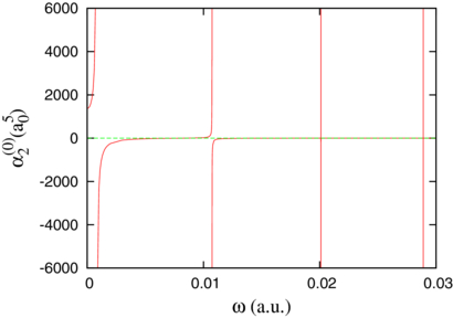
Figure 2. Dynamic quadrupole polarizability α(0)2(ω) for the ground state (0+, 0) of the molecular ion H+2.
Download figure:
Standard imageFor ω = 0, approximation (25) is smaller than the result of table 5 by 4.793. Strikingly, over the ω range of figure 2, this difference remains comprised between 4.79 and 4.80. An extrapolation to v > 3 indicates that, except at resonances, the contribution of higher excited bound states is negligible. We thus interpret the difference between the exact result and approximation (25) as the contribution of the continuum.
3.4. Polarizabilities of the hydrogen molecular ion in a plasma
If we consider the hydrogen molecular ion H+2 immersed in a Debye plasma, then a screening effect appears and the Coulomb potential of the Hamiltonian (4) has to be replaced by [26]

where D is the temperature- and density-dependent Debye length. Using the Lagrange-mesh technique is as easy as for the free case since one only has to replace numerical values of the Coulomb potentials appearing in (4) by numerical values of potential (26) in the code. Table 6 presents the energies E and the static dipole polarizabilities α(L)1 for the four lowest vibrational levels of L = 0 and 1 calculated with the Debye length D = 1. After optimizing the Lagrange-mesh parameters, we use the same number of points for each coordinate Nx = Ny = Nz = 30 and the nonlinear parameters hx = hy = 0.1 and hz = 0.9. Both the energies and the polarizabilities significantly increase with respect to tables 1 and 3. The (0+, 0) ground state result can be compared with the one computed by Kar and Ho [26].
Table 6. Energies, components and averages of the dipole polarizabilities of the molecular ion H+2 placed in a hot plasma for L = 0 and 1 and v = 0 − 3. The Debye length is D = 1. The results are for N = Nz = 30 and h = 0.1, hz = 0.9.
| v |  |
α(0 1)1 | α(0)1 | ||
|---|---|---|---|---|---|
| 0 | −0.045 224 024 1544 | 93.479 429 41 | 31.159 809 80 | ||
| [26] | −0.045 223 | 31.19 | |||
| 1 | −0.039 889 095 0941 | 136.460 0271 | 45.486 675 70 | ||
| 2 | −0.035 215 772 9611 | 195.744 4170 | 65.248 139 03 | ||
| 3 | −0.031 147 0986 | 277.0149 | 92.3383 | ||
| v |  |
α(1 0)1 | α(1 1)1 | α(1 2)1 | α(1)1 |
| 0 | −0.045 039 701 165 7 | 14.762 177 88 | 24.894 288 19 | 54.402 520 66 | 31.352 995 58 |
| 1 | −0.039 724 411 284 0 | 22.545 997 09 | 34.869 374 93 | 79.931 687 71 | 45.782 353 24 |
| 2 | −0.035 069 356 9614 | 33.742 628 | 47.946 493 | 115.379 733 | 65.689 6180 |
| 3 | −0.031 017 615 | 49.798 | 64.826 | 164.334 | 92.9862 |
4. Conclusion
With the Lagrange-mesh method in perimetric coordinates, we have calculated the static dipole polarizabilities of the ground-state rotational band of H+2 for total orbital momenta from L = 0 to 39 with an absolute accuracy of about 10−9. Slightly less accurate results are also given for the first three vibrational excited levels with L = 0 − 2. Some results are given for quadrupole polarizabilities.
The method also allows calculating dynamic polarizabilities without additional difficulty. For the ground state, dynamic dipole and quadrupole polarizabilities are presented. The static dipole polarizability of the hydrogen molecular ion in a Debye plasma is also easily determined with a tiny change in the code.
The theoretical ground-state polarizability is still in disagreement with experiment [3]. An important number of accurate theoretical calculations solving the three-body Schrödinger equation and calculating the ground-state polarizability with a variety of techniques all agree with at least seven significant digits. Relativistic corrections do not seem to cure the problem [13]. Two options remain. Either larger corrections to the Schrödinger approximation exist for some reason, or the experimental error bar is underestimated. For the L = 1 level, there is no discrepancy but the experimental error bar is much larger. It would be helpful to measure polarizabilities of higher levels of the ground-state rotational band, if possible, and to compare them with our accurate results.
Acknowledgments
This text presents research results of the interuniversity attraction pole programme P6/23 initiated by the Belgian-state Federal Services for Scientific, Technical and Cultural Affairs. HOP thanks the FRS-FNRS (Belgium) for a postdoctoral grant.