

Abstract
The classical dynamics of a cold atom trapped inside a static helical optical potential is investigated based on the Lagrangian formalism, which takes into account both the optical light field and the gravitational field. The resulting equations of motion are solved numerically and analytically. The topology of the helical optical potential, which drives the trapped cold atom, is responsible for two different types of oscillations, namely: the local oscillations, whereby the atomic motion is confined in a region smaller than the light field wavelength  and the global oscillations, when the atomic motion is extended to larger regions comparable to the beam Rayleigh range
  Local oscillations guide the atom along the helical structure of the optical potential. The global oscillations, which constitute the main topic of our paper, define the atomic motion along the z-axis as an oscillation between two turning points. For typical values of the beam waist
  the turning points are symmetrical around the origin. For large values of the beam waist
  the global oscillations become asymmetric because the optical dipole potential weakens and the gravitational potential contributes to the determination of the turning points. For sufficiently large values of the beam waist
  there are no global oscillations and only one upper turning point defines the atom's global motion.
Export citation and abstract BibTeX RIS
1. Introduction
The manipulation of atomic translational motion by lasers has been extensively investigated both theoretically and experimentally during the last three decades. This research has led to major achievements in atomic cooling and trapping [1–6] and paved the way for new research fields such as Bose–Einstein condensation and atom optics [6]. The physical basis of these achievements is the interaction of the laser light with the atoms and mainly the linear momentum  associated with a photon, which is absorbed or emitted by the atom. The coherent nature of laser light simplifies this interaction because it involves transitions between a small numbers of internal atomic states. Indeed, the manipulation of the atomic motion involves mostly two internal atomic levels while some very crucial effects, like Sisyphus cooling and velocity selective coherent population trapping involve transitions between three atomic levels [7]. The simplest atom model that can be considered is that of a two-level atom interacting with a coherent light field. It has been shown that such an atom experiences two types of radiation forces: a scattering (dissipative) force due to the absorption-spontaneous emission cycles [8, 9] and a dipole (reactive) force due to absorption-stimulated emission cycles [10]. The latter can be considered, in the limit of small fluctuations, as a conservative force corresponding to the so called optical dipole potential. These forces enable the manipulation of the two-level atoms and they are responsible for effects such as the Doppler cooling, the optical molasses (dissipative force) and the atom trapping (dipole force) [3, 4].
In 1992, in a seminal paper, Les Allen and colleagues have shown that a laser beam with cylindrical symmetry, namely the Laguerre–Gaussian (L–G) beam, possesses an orbital angular momentum of  per-photon, where
  is an integer azimuthal number [11]. When such a beam interacts with a two-level atom it transfers to the atom not only linear momentum but also angular momentum along the beam axis. Thus, the beam exerts a torque on the atom as well [12, 13]. In the saturation limit (very large beam intensity), the maximum torque that can be achieved using a L–G beam is equal to
  where Γ is the natural width of the excited state [12]. Experimentally, Tabosa and Petrov have shown that the OAM of light can be transferred, via optical pumping, to cold cesium atoms [13]. Moreover, the OAM transfer effect has been predicted when a L–G beam is incident on dielectric particles [14]. However, the OAM of light can also be transferred to the internal excitation as well as the rotational motion of cold atom and molecules [15].
Multiple, independent counter-propagating beams in one, two and three-dimensions have been considered to study the dynamics of a  ion due to the OAM transfer [16, 17], or to achieve a Doppler cooling if the counter-propagating beams have opposite helicities [18]. Recently, the use of properly tailored light masks, made by superposition of L–G beams with tilted plane waves, has been proposed as suitable diffraction masks for the generation of atom vortex beams [19]. Different schemes for the generation of atom vortex states for trapped BECs have been also proposed. In particular, a vortex state can be created by transferring the light's angular momentum to the BEC using two co-propagating
  and
and  polarized L–G beams in a Raman transition [20]. Moreover, the creation of a vortex state was also proposed by using four traveling-wave laser beams [21]. The four beams can be controlled to form a harmonic trap to induce quantized circular motion to a BEC [22]. Finally, a suitable dipole potential was formed using four traveling-wave laser beams with Gaussian or L–G transverse profiles to generate a skyrmion in a spinor BEC [23].
The use of twisted beams carrying OAM has been shown to be very important for the generation of artificial gauge magnetic fields both in schemes involving the interaction of two- and three-level atoms with L–G beams in the free space [24] as well as with evanescent light fields with phase singularities [25]. We must point out that L–G beams have been proposed as higher-dimensional quantum systems that can be used in quantum communications and quantum cryptography [26].
One of the most spectacular achievements of atom trapping in structured light fields is the optical lattice. An optical lattice that can be formed by the interference of pairs of counter-propagating plane waves or structured beams in one, two and three-dimensions is a periodic geometrical pattern of high and low intensity regions [4, 6]. Cold atoms can be manipulated by being trapped either at high (in red detuned light  or low intensity regions (in blue detuned light
  of the lattice. Optical lattices enable the investigation of many effects in condensed matter such as the quantum phase transition from a superfluid to Mott insulator [27] and the realization of arrays of Josephson junctions [28].
The beams with photons carrying OAM have opened up new opportunities for the generation of optical lattices with a cylindrical symmetry. A two-dimensional static or rotating optical ring lattice (optical Ferris wheel) has been demonstrated at the focal plane of co-propagating L–G beams with different l-indices [29]. The optical ring lattice can be either a bright ring suitable for trapping atoms in red-detuned light or a dark one suitable for trapping atoms in blue-detuned light [29]. The three-dimensional structure of two counter-propagating L–G beams with opposite l-indices has a helical shape (twisted tubes). A superfluid ensemble trapped in a rotating helical optical tube has been shown to be associated with an artificial magnetic field [30]. The twisted tubes can be considered as a waveguide for atomic motion in distances far smaller than the Rayleigh range of the beam  [31], while connections between Gaussian lattices and helical optical tube have been also considered in the same work [31].
The structure of this paper is as follows: the derivation of the helical dipole potential is described in section 2, while in section 3 we study the atomic motion in the helical tube potential. In section 4 we describe the numerical model and the parameters of our calculations. In section 5, which includes two subsections, we describe the analytical calculations. In section 5.1 we investigate the topological features of the helical dipole potential at different scales. In section 5.2 we present the analytical calculation for the atomic motion in the region  to obtain the global atomic oscillation. The results for the total atomic motion inside the helical potential, using both numerical and analytical calculations, are presented in section 6. The turning points of the global oscillation and their relation to various parameters of the dipole potential such as: the power of beam P, the beam frequency detuning Δ, and the beam waist
  are studied in section 7. Finally, in section 8 we present our conclusions.
2. The helical optical potential tubes
The twisted optical potential tubes are formed by the interference of two counter-propagating L–G beams, with opposite helicities  and the same polarization, that results in the generation of a standing wave. The electric field of a L–G beam of power P, which is considered as linearly polarized along the x-direction and propagates along the z-axis is given by:
In equation (1) the quantity  is given by
where  is an associated Laguerre polynomial and
  is the beam waist at position z, where
  is the beam waist at
  and
and  is the Rayleigh range, which is equal to
  with
with  the wavelength of the beam. The two last exponential terms in equation (2) are the so called curvature and Gouy phases respectively [17].
If we consider the Gouy phase and curvature terms as negligible sine we are going to consider small beam helicity and work close to the beam focus, then two counter-propagating terms of opposite helicity when interfere will produce an optical field with the following intensity

where  is the intensity of one of the two beams.
When such a light field is far detuned with respect to an atomic transition, the dissipative force on the atom is suppressed and the optical dipole force is dominant. Τhis force is conservative and it is attributed to the optical dipole potential which has the simple form

with  being the Rabi frequency and
  the excited state spontaneous emission rate. The atom dynamics can be described as a result of the action of forces (semiclassical approximation) in the case where the characteristic time of external variables
  (
( is the radiative life time), or the single photon recoil energy
  (
( is the atomic linewidth) [6].
The relation between the Rabi frequency and the intensity of the laser field [4] is:

with  being the saturation intensity which depends on the specific atomic transition chosen.
Using equations (3)–(5) by considering the case of static optical tubes we get:

Figure 1 shows the helical optical tube dipole potential for a mode with  and
and  This pattern has a left-handed helical shape with a pitch equal to
 Moreover, the three-dimensional optical dipole potential includes two tubes where the maximum intensity is at the center of each tube at
  However, the intensity at each tube decreases as you move radially away from the center of each tube, and away from
  along each tube.

Figure 1. The helical optical tube with mode l = 1 and p = 0.
Download figure:
Standard image High-resolution image3. Study of the atomic motion in the helical tube potential
We proceed now in the semiclassical study of a two-level atom inside the optical potential described above. The semiclassical approximation allows us to treat the external variables classically. We consider that the atom is subjected to the optical dipole potential and the gravitational potential. The Lagrangian of an atom inside these two fields in cylindrical coordinates is written as follows:

Since the Lagrangian is not explicitly time dependent, we can use the Euler–Lagrange equations to write the equation of motions:


4. Numerical solution estimation of atom trajectory
The above three equations of motion are coupled nonlinear differential equations of the second order for which it is very hard to find an exact analytical solution. We can solve these equations numerically using the fourth order Runge–Kutta method.
The initial conditions for the cold atom inside the helical optical tube are very important in order to solve the equation of motion. If the light field is red detuned with respect to the atomic transition  then the atom is attracted by the potential well towards the high intensity regions. The initial position of the cold atom can be chosen at the maximum intensity point (which is the minimum value of the dipole potential). The initial position in cylindrical coordinates is:
where  is the index of the tubes of the helical optical potential. For example, if
  then the helical optical potential has two tubes: the first tube has index
  while the second one has index
  (see figure 1). However, the initial velocity of the cold atom should not be chosen to be less than the recoil velocity
  (in order to ensure the validity of the semiclassical approximation) and greater than the Doppler velocity
  (so as to keep the interaction resonant), i.e.
  .
.
5. Analytical expression for the atomic trajectory
5.1. The topology of the helical dipole potential
In this paragraph we arrive at an analytical expression for the atomic trajectory. For simplicity let us choose  (where
  Then the dipole potential is given by:
The term  is responsible for the formation of 2l potential wells (each well corresponds to a tube in the potential depicted in figure 1) in the z − φ plane (see figure 2(a)). Each of these wells has minima along the line
  (n is the index of the tube of the potential). Due to this topological feature of the dipole potential the atom oscillates locally about the line
  which is the locus of the minima of the potential wells. As we may see from figure 2(a), the ranges of oscillations are:
  and
and  The local oscillations will induce an average motion along the line
  which will guide the atom inside the tube of index n by keeping
  and a radial distance
  This guiding will elevate the atom along the z-direction.
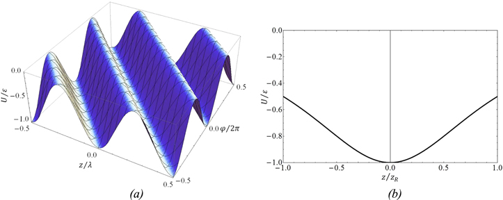
Figure 2. (a) The reduced dipole potential of the helical optical tube as a function of  and z, at a radial distance
  (b) The scaled (in units of its maximum depth
  twisted optical dipole potential as a function of z along the minima line
  .
.
Download figure:
Standard image High-resolution imageAlong the z-direction the motion has another interesting feature: due to the factor  the depth of the potential along the minima line is modified as it may be seen from figure 2(b). It is straightforward to understand that if the kinetic energy of the atom is less than the depth of the dipole potential in this larger scale, the atom will perform a global oscillation between two turning points. Thus the motion inside the twisted optical potential tubes is made up of two 'component' motions: a local atomic oscillation in the region
  and
and  and a global oscillation in the region
  The two types of motion are due to the fact that the dipole potential has two different topological features with different spatial scales.
5.2. Global atomic oscillation
The calculations of Bhattacharya [31] showed that the atom performs local oscillations within distances  with frequency
  and a radial wiggling motion around the radial minima
  of the dipole potential with frequency
  (where
  is the single photon recoil energy,
  is the pitch angle, and
  is the depth of dipole potential at the minimum point).
The atomic motion within  along the minima of the nth tube of the optical potential (with a left-handed helicity) unfolds while
  is equal to one. Consequently, the best way to represent the atomic motion along the minima of the nth tube is to use the helix parameterization
  Using this parameterization, the cylindrical coordinates of the left-handed helix are expressed as:

The dipole potential energy can be now written as:

and ε is the depth of dipole potential at the minimum point (red detuning case):

Moreover, the kinetic energy can be written as:
where  and
and  However, since our interest is
  then
then  which implies that
  and leads to
If we use the following definitions


then the kinetic energy will take the following simple form

Our assumption is that the atomic radial wiggling does not have a strong effect on the global oscillations. This assumption is corroborated by our numerical calculations. As shown in figure 3, for different initial conditions that either result in radial wiggling motion (black line) or not (dashed line), the upper turning point of the global oscillation is unaffected. This is true for a large range of values of the beam waist. Even for a beam waist as large as  the deviation of the turning points with and without radial wiggling is of the order of 3.6%. Therefore, our assumption to ignore the radial wiggling motion in our analytical derivation of the global oscillations is well justified.
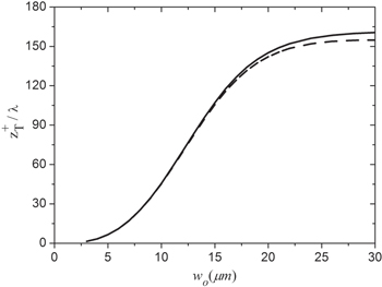
Figure 3. Variations of the upper turning point of the global oscillation versus the beam waist. The black line corresponds to initial conditions that result in radial wiggling motion while the dashed line is obtained with initial conditions for which no wiggling motion is obtained. The two lines start to deviate at approximately  The deviation is 3.6% for the maximum value of the beam waist tested, namely
  .
.
Download figure:
Standard image High-resolution imageConsequently, the total mechanical energy of the global oscillation depends only on one helix parameter ξ and of course is conserved. Thus, the total mechanical energy can be used to obtain the equation of motion for the global oscillation. From the total mechanical energy, we can obtain the following nonlinear differential equation:

where  is the total energy of the atom at the initial point.
The integration of the nonlinear differential equation (20) is difficult. However, 
 Since
Since  for different values of the beam waist, then the right-hand side of equation (20) can be approximated to the second order of the parameter
  to get:
It can be shown that this equation takes the final form

where  and
and  is the frequency of the global oscillation:
where  is the initial angular kinetic energy of the atom which is much smaller than the depth of the dipole potential
  Equation (23) helps us clarify the effect of the helical structure of dipole potential and the number of helical tubes
  on the strength of the trapping in the helical optical Ferris. For
  then
then  which implies that the value of the global trapping frequency is much smaller than the local trapping frequency
  and radial trapping frequency
  .
.
The initial position coordinates of the atom,  and
and  imply that
  thus equation (22) can be integrated as follows:

We can use the following integration formula [32]:
where  and
and  The equation of motion of the global oscillations that is obtained from the solution of equation (24) is:
where the subscript G denotes the global oscillation, and  is a phase shift due to the effect of gravity:

Now, we can obtain the global oscillation along the φ- and z-directions using  and
and  respectively. Moreover, the full solution along the φ- and z-directions can be constructed by using Bhattacharya results [31] as
  and
and  :
:
In order to describe the radial wiggling  about the radial minima
  (such that
  along the whole atomic trajectory we will use the Bhattacharya results [31] and the initial conditions to get:

This equation shows clearly that the radial motion is an oscillation about the radial minima potential positions.
6. Results
In figure 4 we present the three-dimensional trajectory of a 85Rb atom that has been numerically calculated (see figure 4(a), red line) and analytically, using the equations (28)–(30), (see figure 4(b), blue line).
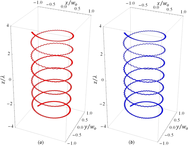
Figure 4. The 3D trajectory of 85Rb atom along the helical tube with index  with a time duration of
  calculated: (a) numerically (red line) and; (b) analytically (blue line).
Download figure:
Standard image High-resolution imageThe parameters that are used in both methods are for a 85Rb atom where the light field excites the transition  characterized by the following parameters:
  Is = 1.64 mW cm−2, and
  [4]. The recoil and Doppler velocities for laser cooling of a 85Rb atom are
  and
and  respectively [4]. The parameters of the L–G beam that are used for trapping a 85Rb atom are: power
  detuning
  [33], and beam waist
  The figures 4(a) and (b) show an excellent agreement between the numerical and analytical calculations. Both figures show the global oscillatory behavior of a 85Rb atom between two turning points along the z-axis and following a helical trajectory due the helical geometry of the dipole potential.
7. Turning points
The turning point is one of the important features of the trajectory of the atom inside the twisted optical tube. It defines the furthest point the atom can be guided along the helical optical tube. Additionally, the turning point is a parameter of the atomic gross motion that can be manipulated by changing the parameters of the involved L–G beams. We can consider the conservation of energy which implies that the total energy of the atom at the initial point equals to the total energy at the turning point:

If we multiply this expression by  and using
  and
and  for the turning point, we get a cubic equation:

where 
 and
and  .
.
The roots of the cubic equation (32) can be found numerically. One of the real roots of this cubic equation is positive while the other one is negative. The positive root corresponds to the upper turning point of the atomic motion while the negative one to the lower turning point. The positive and negative roots, as obtained analytically, are depicted by the blue and yellow lines, respectively, in figures 5–7. The red squares and the green triangles represent the upper and lower turning points, respectively, as obtained from fully numerical calculations. The results from both methods of calculation of the turning points agree very well. Moreover, figures 5–7 show that the upper and lower turning points can be manipulated by changing certain beam parameters such as: the beam power (see figure 5), the detuning Δ (see figure 6) and the beam waist  (see figure 7). Additionally, the upper turning point of the atom can be higher if the dipole potential becomes weaker by making: the beam waist
  larger, the beam power smaller or the detuning Δ larger. On the other side, the lower turning point of the atom is lower and farther than the upper turning point if the dipole potential becomes weaker.
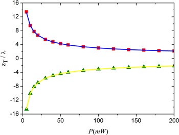
Figure 5. The variation of the upper turning point (fully numerical results depicted by red squares and analytical ones by the blue line) and the lower turning point (fully numerical results depicted by green triangles and analytical ones by the yellow line) with beam power for a 85Rb atom with initial velocity  (where
  and
and  ).
).
Download figure:
Standard image High-resolution image
Figure 6. The variation of the upper turning point (fully numerical results depicted by red squares and analytical ones by the blue line) and lower turning point (numerically by green triangles and analytically by yellow line) with detuning for a 85Rb atom with initial velocity  (where
  and
and  ).
).
Download figure:
Standard image High-resolution image
Figure 7. The variation of the upper turning point (fully numerical results depicted by red squares and analytical ones by the blue line) and lower turning points (fully numerical results depicted by green triangles and analytical ones by the yellow line) with beam waist for a 85Rb atom with an initial velocity  (where
  and
and  ).
).
Download figure:
Standard image High-resolution imageAdditionally, the values of the lower and the upper turning points are symmetric with respect to the origin when the dipole potential is strong and therefore the influence of gravity negligible. However, the asymmetry between the values of the lower and the upper turning points (where the lower turning point becomes more distant from the origin than the upper turning point) is evident as the dipole potential becomes weaker and gravity affects the atomic motion significantly.
However, figure 7 shows that if the beam waist is  the upper turning point does not change. This saturation in the value of the upper turning point is due to the fact that the gravitational force becomes dominant and the dipole force insignificant. Indeed, if the beam waist becomes large, then the ratio
  and the first two terms of equation (32) tend to zero:

Equation (33) shows that the atom is solely under the influence of gravity. The initial velocity in our case is  thus the maximum turning point of the motion is
  which agrees with the result in figure 7.
Focusing on figure 7 one can conclude that at small beam waists the atom trajectory has two symmetric turning points (the upper and the lower one) due to the strong dipole force. However, as the beam waist increases the dipole force becomes considerably weaker (because the effective potential varies as  and in this case the trajectory has two asymmetric turning points. Moreover, for even larger beam waists the motion of the atom, governed almost entirely by the gravity, has only one turning point. Its initial velocity allows the atom to move up and reach the upper turning point, then the atom starts to fall under the influence of gravity 'only' and follows in its downward motion the helical path determined by the topology of the optical tubes. Consequently, the number of real roots of the cubic equation (equation (32)) can tell us which parameters are suitable in order to keep the atom oscillating between the turning points. The number of real solutions of a cubic equation depends on the value of the following discriminant [34]:

Specifically, we obtain:
- (1)Three real roots if
 two of which correspond to the two turning points, one corresponding to the positive root and one to the negative one, while the third root has a very large negative value.
 - (2)Two identical negative roots and one positive root if In this case, we get different absolute values for the negative and positive roots, which correspond to two asymmetric turning points.
- (3)Two complex roots and one real root if The real root corresponds to a single turning point.


The value of beam waist for which  is called critical beam waist
  If the value of the beam waist is smaller than
  then
then  while for beam waist larger than the critical value
  .
.
Figure 8 shows the change in the potential energy  as a function of
  for different values of the beam waist:
  (blue solid line),
  (red dashed line), and
  (green dotted line). The dashed black line represents the initial kinetic energy of the atom
  When the beam waist is equal to
  the initial kinetic energy of the trapped atom
  intersects the potential energy curve only at two points
  (negative z) and
  (positive z), which means that this value of the beam waist is the critical value
  The values of the initial kinetic energy and
  are equal at the turning point
  which is the maximum turning point that the atom can reach along the negative z direction while the atom is still under the influence of the dipole potential:

However, if  (green line) then
  and the atomic motion has only one turning point because the effect of gravity on the atom is dominant. Moreover, if
  (blue solid line) then
  and the atomic motion has two turning points because the effect of the dipole potential on the atom is dominant. In this case (figure 8, blue solid line), we also obtain a third real negative root with large absolute value. It corresponds to an initial position of the atom for which its motion is unbounded. More specifically, the atom is trapped between the upper and lower turning points only if its initial position has a z-coordinate lying between the values of the two turning points. The range between the two negative roots of the third-order equation (32) is classically forbidden for the atom. Finally, if its initial position has a z-coordinate corresponding to the second negative root or smaller, then its motion is unbounded along the negative z-axis. Similar remarks can be presented for the other two cases, although their interpretation is more straightforward.

Figure 8. The values of initial kinetic energy of the trapped atom  (black dashed–dotted line) and the difference of potential energy
  for different values of the beam waist:
  (blue solid line),
 (red dashed line), and
  (green dotted line). The dipole potential parameters are
  and
and  Τhe atom's initial velocity components are
  .
.
Download figure:
Standard image High-resolution image
8. Conclusions
We studied, in great detail, the classical motion of a two-level atom inside a twisted optical dipole potential formed by two counter-propagating L–G beams of opposite helicity. The analysis is based on the Lagrangian formalism and thus is amenable to extension to a quantized description of the atomic motion, which we leave for a future publication.
The atomic motion inside the helical optical tube can be described in terms of three different oscillations: a local oscillation, a global oscillation, and a radial wiggling oscillation. The frequencies of the local oscillation  and the radial oscillation
  were predicted by Bhattacharya [31] to obey
  a result that is corroborated by our results. The local oscillation creates a strong coupling between the z- and φ-components of the atomic velocity, which induces global motion along the helical tube. However, the global oscillation along the helical tube has a frequency
  much smaller than the other frequencies. These motions were investigated both numerically and analytically and we found an excellent agreement between these two methods.
The frequencies of all oscillations inside the helical tubes and the values of turning points can be manipulated at will by changing certain parameters of the optical beams such as: the beam waist  the beam power and the wavelength (which directly affects the detuning Δ of the atomic dipole transition).
When the dipole potential is dominant (negligible gravity effect), the trapped atom will oscillate between the symmetrical positions of the upper and lower turning points, a situation equivalent to an atom reflected between two perfect mirrors of an atomic cavity. However, the strength of the dipole potential can be manipulated by changing the optical parameters to let the effect of gravity become significant and convert the lower mirror of the atomic cavity to a partially transmitting one, allowing for a controlled leakage of atoms trapped in the potential. A full quantum mechanical study of the set-up will reveal to what extent it can be used as an atom 'laser'.
The calculations have revealed an upper limit in the value of the upper turning point (for given beam power and the detuning Δ). In this case, the value of the turning point does not change as the beam waist increases. This limiting behavior of the upper turning point is due to the fact that the gravitational force becomes dominant and the dipole force cannot manipulate any further the atomic motion.
When the gravitational force is dominant the atomic motion has only one tuning point. On the contrary, it has two turning points, and motion inside the tubes is ensured, if the dipole force is dominant. We can use the twisted optical tube with large value of beam waist  as a sensor of any change in the value of the gravitational acceleration
  that can be obtained from equation (33) and the value of the upper turning point
  such that
  .
.
Finally, the helical optical tubes can be used as an atomic guide against the effect of gravity to the desired elevation by changing the parameters of the optical potential. On the contrary, the dark hollow beam is used to guide an atom with the help of gravity with always downward direction, a situation corresponding to an atom funnel [35].
Acknowledgments
We thank Professor Peter Zoller for useful and stimulating discussions. This project was funded by the National Plan for Science, Technology and Innovation (MAARIFAH), King Abdulaziz City for Science and Technology, Kingdom of Saudi Arabia, Award Number (11-MAT-1898-02).