
Abstract
Recent technological advances in the generation of intense femtosecond pulses have made covariance mapping an attractive analytical technique. The laser pulses available are so intense that often thousands of ionisation and Coulomb explosion events will occur within each pulse. To understand the physics of these processes the photoelectrons and photoions need to be correlated, and covariance mapping is well suited for operating at the high counting rates of these laser sources. Partial covariance is particularly useful in experiments with x-ray free electron lasers, because it is capable of suppressing pulse fluctuation effects. A variety of covariance mapping methods is described: simple, partial (single- and multi-parameter), sliced, contingent and multi-dimensional. The relationship to coincidence techniques is discussed. Covariance mapping has been used in many areas of science and technology: inner-shell excitation and Auger decay, multiphoton and multielectron ionisation, time-of-flight and angle-resolved spectrometry, infrared spectroscopy, nuclear magnetic resonance imaging, stimulated Raman scattering, directional gamma ray sensing, welding diagnostics and brain connectivity studies (connectomics). This review gives practical advice for implementing the technique and interpreting the results, including its limitations and instrumental constraints. It also summarises recent theoretical studies, highlights unsolved problems and outlines a personal view on the most promising research directions.
Export citation and abstract BibTeX RIS

Original content from this work may be used under the terms of the Creative Commons Attribution 3.0 licence. Any further distribution of this work must maintain attribution to the author(s) and the title of the work, journal citation and DOI.
1. Introduction
Covariance mapping is a generalisation of covariance, which is a scalar that measures a statistical relationship between two random variables. Covariance maps are matrices that show statistical relationships between different regions of random functions. The maps show statistically independent regions of the functions as zero-level flatlands, while positive or negative correlations are depicted as hills or valleys, respectively.
The effectiveness of covariance mapping arises from the fact that the mathematics conveys physical meaning. For example, when the random functions are time-of-flight (TOF) spectra of molecular fragment ions produced in a process of dissociative ionisation, the hills on the covariance map reveal the fragmentation paths of the parent ions. Even if the parent ion is unstable and not observed on the normal, one-dimensional (1D) TOF spectrum, the covariance map reveals its presence. Moreover, knowledge of the fluctuation statistics (which are normally Poissonian for gas-phase experiments) allows us to interpret the covariance map quantitatively.
Covariance mapping techniques are particularly suitable for analysing experimental spectra at free-electron laser (FEL) facilities, where very intense radiation induces hundreds or thousands of ionisation events at each laser pulse. Such high counting rates overwhelm simpler coincidence techniques and render them unsuitable for FEL research. In principle, covariance mapping can cope with arbitrarily high counting rates, but in practice there are limitations. This has led to the development of more advanced versions, such as partial covariance.
This article starts with the historical origins and summarises the initially modest use of the covariance mapping technique. This is followed by a detailed description of the simple and partial techniques, before concluding with a review of the recent expansion of research activity in this area.
1.1. History of covariance mapping
The precursor of covariance mapping is the triple coincidence technique to analyse dissociative double ionisation processes induced by a high energy photon, either in a direct process or via Auger decay. In the photoelectron–photoion–photoion coincidence technique [1, 2], detection of one of the photoelectrons provides a start time from which the TOF of subsequent fragment ions is measured. Pairs of these TOF measurements form the coordinates of points that are added to an ion–ion coincidence map. With a pulsed source of photons, such as radiation from a synchrotron operating in the single-bunch mode, it is also possible to time the photoelectrons and accumulate a photoelectron–photoion TOF coincidence map [2].
Coincidence techniques produce clean maps, provided the counting rate is low enough that the probability of more than one event occurring within the TOF window is negligibly small. Any extra events spoil the map by creating a structured background of false coincidences. The motivation for devising the first covariance mapping technique [3] was a desire to capture and remove this background using the mathematical formula of covariance. The technique successfully unravelled the dynamics of multiphoton multiple ionisation in intense picosecond laser fields for a series of molecules: CO, N2O, SO2 [3], N2 [4] and I2 [5], and demonstrated that at long photon wavelengths (visible and infrared) the fragmentation follows predominantly charge-symmetric channels [6]. Covariance mapping has also been used for studying pathways of molecular fragmentation induced by electron impact [7, 8], nuclear magnetic resonance spectroscopy [9], and even for welding diagnostics [10].
Covariance mapping bears similarities to two-dimensional infrared (2D-IR) spectroscopy in the condensed phase. It seems that the two techniques have been developed independently. Initially the 2D-IR technique was quite dissimilar, requiring a sinusoidal external perturbation to induce molecular changes [11]. Later, however, this technique was generalised to an arbitrary perturbing waveform, which created an explicit connection with the covariance formula (equations (17) and (18) in [12]). Currently, the synchronous 2D-IR technique effectively produces the same result as covariance mapping, albeit with a more complex excitation scheme [13, 14].
2. The principle of covariance mapping
To illustrate how covariance mapping works, we can examine the experimental setup shown in figure 1. In this experiment, x-ray pulses are focused on neon atoms and ionise them. The kinetic energy spectra of the photoelectrons ejected from the atoms are recorded at each laser shot using a suitable spectrometer (here, a TOF spectrometer). The single-shot spectra are sent to a computer, which calculates and displays the covariance map.
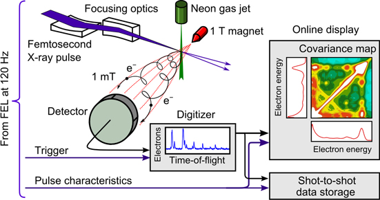
Figure 1. Schematic of a covariance mapping experiment, performed at the LCLS FEL at Stanford University. Figure reprinted from [15]. © 2013 American Physical Society.
Download figure:
Standard image High-resolution image2.1. The need for finding correlations
Even in a relatively simple system such as the neon atom, intense x-rays induce a plethora of ionisation processes (see figure 2). Since the kinetic energies of the electrons ejected in different processes largely overlap, it is impossible to identify these processes using ordinary 1D photoelectron spectrometry. To do so, one needs to correlate the kinetic energies of the electrons belonging to the same process, and covariance mapping is a method of revealing such correlations.
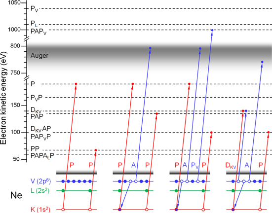
Figure 2. Ionisation processes in neon induced by intense x-ray photons of 1062 eV energy. The four diagrams show examples of competing electron ejection sequences. The colours indicate the origin of the electrons: the atom core (K, red), the inner valence shell (L, green) or the valence shell (V, blue). In the first diagram (PP), absorption of a photon ejects a photoelectron (P) from the core (the first arrow) and creates a core hole (an open circle). Before the hole is filled, another photon is absorbed and the second core electron is ejected. The kinetic energy of the two electrons is shown on the vertical scale: it is lower for the second photoelectron in the PP sequence because the first electron no longer screens the nucleus. (The energies of the K, L, V shells are not drawn to scale). However, before the second photoelectron is ejected, an Auger process may occur as shown in the second diagram (PAP): an electron from the valence shell fills the first core hole and ejects an Auger electron (A) from the valence shell. Subsequently, when the next photoionisation occurs (the second P), the first core hole is already filled; there is more screening and the kinetic energy of the second photoelectron is higher for the PAP process than the PP one, as indicated by the dashed lines and their labels on the vertical scale. The third diagram (PAPVP) shows that additional photoionisation from the valence shell (PV) may interrupt the PAP sequence and reduce the kinetic energy of the last photoelectron. The fourth diagram (DKVAP) depicts a process where a core photoelectron on its way out (the first red arrow) may also kick out an additional valence electron (the first blue arrow) giving a double electron ejection by a single photon (DKV). Generally, there are many more sequences of electron ejections present at high x-ray intensities, some of them also involving the green inner valence shell. Figure reprinted from [15]. © 2013 American Physical Society.
Download figure:
Standard image High-resolution image2.2. Simple covariance mapping
Consider a random function Xn(E), where index n labels a particular instance of the function and E is the independent variable. In the context of the FEL experiment, Xn(E) is a digitised electron energy spectrum produced by laser shot n. As the electron energy E takes a range of discrete values, Ei, the spectra can be regarded as row vectors of experimental data:
where italics denote scalars and bold type is used for vectors (and matrices later on). The simplest way to analyse these data is to average the spectra over N laser shots:
Such spectra show the kinetic energies of individual electrons but the correlations between the electrons are lost in the process of averaging. To reveal the correlations we need to calculate the covariance:
where vector Y = XT is the transpose of vector X and the angular brackets denote averaging over many laser shots, as in equation (2). Note that the ordering of the vectors (a column followed by a row) ensures that their multiplication gives a matrix. It is convenient to display the matrix as a colour map.
2.3. Map interpretation
The covariance map obtained in the FEL experiment illustrated above [15] is shown in figure 3. Along the x and y axes are shown the averaged spectra 〈X〉 and 〈Y〉. On the map these spectra are resolved into pairwise correlations between the energies of electrons coming from the same process. For example, if the PP process shown in figure 2 occurs, then two low-energy electrons are ejected from the Ne core giving a positive island in region (a) of the map. The positivity of the island is due to statistical fluctuations of the number of atoms undergoing the PP process at each shot: if more (fewer) electrons are ejected in the first ionisation step, then more (fewer) electrons are likely to be produced in the second step as well, which gives a positive contribution to the covariance between the two electron energies irrespective of the sign of each fluctuation.

Figure 3. A covariance map revealing correlations between electrons emitted from neon (and from some N2 and water vapour contamination). The map is constructed shot-by-shot from electron energy spectra recorded at a photon energy of 1062 eV, which are shown along the x and y axes after averaging over 480 000 FEL shots. Volumes of the features on the map give relative probabilities of various ionisation sequences, which can be classified as: (a) Ne core–core; (b) H2O core–core, core–Auger, and Auger–Auger; (c) Ne Auger–Auger; (d) Ne valence–valence; (e) N2 core–Auger; (f) H2O core–valence; (g) Ne core–Auger; (h) Ne core–valence; (i) double Auger and secondary electrons from electrode surfaces; and (j) Ne main (core) photoelectron line. The colour scale is nonlinear to accommodate a large dynamic range. Figure reprinted from [15]. © 2013 American Physical Society.
Download figure:
Standard image High-resolution imageOne consequence of using a single detector and taking Y = XT is the mirror symmetry of the covariance map, since in this case cov(Ex, Ey) = cov(Ey, Ex). Another feature is the diagonal autocorrelation line, which occurs simply because an electron pulse present on a spectrum at Ex is always present at Ey. The values along the ridge of the autocorrelation line on the map are given by the variance 〈X2〉 − 〈X〉2 of the spectra, and the shape of a cross section of the ridge reflects the instrumental energy resolution.
If the experimental conditions are held constant (in particular, if every laser pulse is the same), then the volumes of the islands are directly proportional to the relative probabilities of the ionisation processes [3]. This quantitative aspect of the map follows from a property of the Poisson distribution, which characterises the number of neon atoms in the focal volume and the number of electrons produced at a particular energy Xn(Ei). The property employed states that the variance of a Poisson distribution is equal to its mean, and this property is also inherited by covariance. Therefore, the covariance plotted on the map is proportional to the number of neon atoms that produce pairs of electrons at particular energies. This makes covariance much more suitable for particle counting experiments than other bivariate estimators, such as Pearson's correlation coefficient.
2.4. Inner-shell processes revealed
Much more information is present on the map than on the averaged 1D spectrum. Single, often broad and indistinct peaks on the 1D spectrum are resolved into several islands on the map. Figure 4 shows magnified core–core and core–valence regions with several ionisation sequences unambiguously identified. In a DKV process the two ejected electrons arbitrarily share the energy available from a single photon, producing a conspicuous line at Ex + Ey = const in the left panel of figure 4. Impurities, such as water vapour or nitrogen, form islands that are usually found away from the correlation structures of the species under analysis (see figures 3(b), (e) and (f)).

Figure 4. Identification of neon ionisation processes in the core–core (left) and core–valence (right) correlation regions. The top of the autocorrelation line is cut off to show the features behind. The process labels are explained in the caption of figure 2. The two detected electrons giving rise to the covariance signal are indicated by bold type. Figure reprinted from [15]. © 2013 American Physical Society.
Download figure:
Standard image High-resolution imageCovariance maps reveal not only the energies of electrons ejected in the same ionisation process but also the relative yields of these processes, which are proportional to the island volumes. This information allows us to quantitatively compare the experiment with theory [16].
2.5. Coincidences from covariance mapping
The triple coincidence technique [1, 2] is a special case of covariance mapping suitable for low counting rates, i.e. when only a few particles at most are typically detected at each laser shot and the probability of two arriving at the same TOF can be neglected. To make data processing efficient, such sparse single-shot spectra are normally passed through a discriminator, which sets the X and Y values to either 0 or 1 and reduces equation (3) to the coincidence formula:
where N is the total number of laser shots fired during the experiment, including those shots where no particle was detected. The first term of equation (4) is the basic map of the number of coincidences in the TOF spectra. The second term is the background of false coincidences and it is negligibly small if the counting rate is low (≪1 event per shot). However, for moderate counting rates (a few events per shot but with the probability of more than one particle arriving within the same TOF sample still negligible) this second term should be taken into account.
3. Partial covariance mapping
In practice, the assumption of constant experimental conditions made in section 2.3 is rarely possible. Covariance maps often display all kinds of correlations, including indirect ones induced by a fluctuating common parameter. Such common-mode correlations are often uninteresting and they obscure the interesting ones. For example, in laser-based experiments the pulse intensity may fluctuate from shot to shot, which correlates every electron with every other electron simply because a more intense pulse produces more electrons at any energy.
3.1. The principle
The influence of such uninteresting correlations can be removed using partial covariance mapping, which was proposed some time ago [17] but implemented only recently. The method requires knowledge of the fluctuating parameter I, which must be measured at each laser shot. Calculating the covariance of this parameter with the TOF spectrum allows us to estimate the contribution of fluctuations in I to the covariance map and subtract this contribution from the map. The rigorous derivation of the partial covariance formula is lengthy [18] but the result is quite simple:
where cov(I, I) is the variance of the fluctuating parameter.
The second term in equation (5) is the correction to the simple covariance map, cov(Y, X). Note that cov(Y, I) and cov(I, X) are a column and a row vector respectively, so their product gives a matrix. The division by cov(I, I) ensures that the correction is independent of the amplitude of the parameter fluctuations and that the units are consistent. The partial covariance map, pcov(Y, X; I), shows only a part of the correlations: the part that is independent of I. The end result is that partial covariance map shows correlations as if the fluctuating parameter was held constant during the experiment.
3.2. Stages of partial covariance mapping
While partial covariance mapping was also used to analyse the LCLS experiment in [15], to see how it works it is more instructive to consider another experiment, performed at the FLASH FEL in Hamburg. The FLASH experimental setup was very similar to the LCLS setup shown in figure 1, except that molecular nitrogen was studied and ions, rather than electrons, were detected [19]. Figure 5(a) shows the correlated product 〈YX〉 and figure 5(b) shows the uncorrelated product 〈Y〉〈X〉. Their difference gives the simple covariance map (c). The momentum correlation lines start to be visible here (note a change in the range of the colour scale) but the map is overwhelmed by correlations induced by FEL intensity fluctuations. These correlations are calculated in panel (d) and the correction is subtracted from map (c) to give map (e). The momentum correlation lines are now clearly visible but some residual common-mode background is still present, producing positive rectangles with the momentum lines on their diagonals. This background is likely to be induced by other fluctuating parameters, such as the sample density or the FEL pulse duration. As these parameters were not monitored their magnitude was unknown, therefore simply an excess of the correction (d) was subtracted from map (e), giving map (f). The criterion for the amplitude of this correction was to suppress the rectangular background in the vicinity of a chosen momentum correlation line. This crude, ad hoc method significantly suppresses the residual common-mode background in the region of interest but the overcorrection introduces negative regions (magenta) at long times of flight. The detailed algorithm for partial covariance mapping is given in the Supplemental Material of the LCLS paper [15].
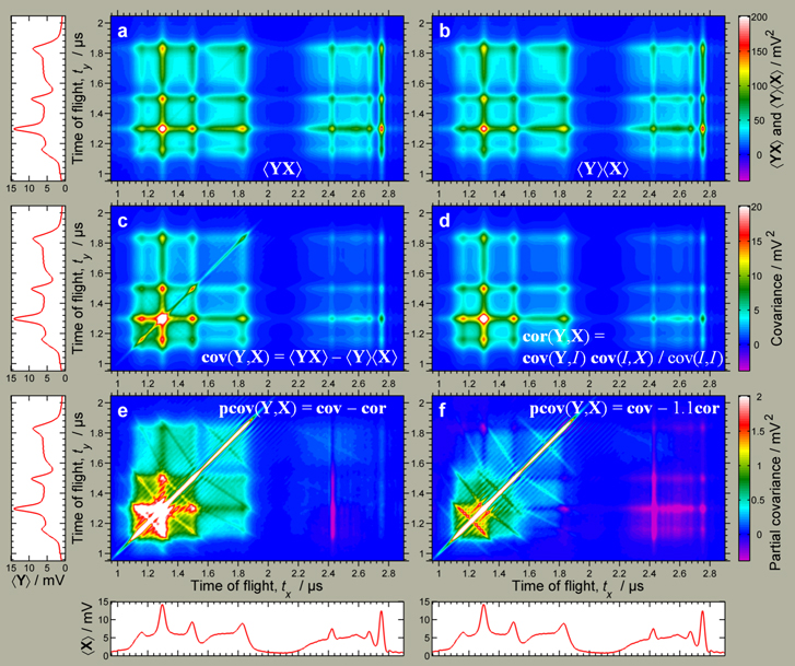
Figure 5. Stages of partial covariance mapping to resolve the ion momentum correlations in the Coulomb explosion of N2 molecules. Owing to momentum conservation these correlations appear as lines approximately perpendicular to the autocorrelation line (and to the periodic modulations which are caused by detector ringing). Figure reprinted from [19]. © 2013 IOP Publishing Ltd.
Download figure:
Standard image High-resolution image3.3. Coulomb explosion dynamics
While the 1D TOF spectra (shown in the side panels of figure 5) are difficult to interpret due to broad, overlapping peaks, the partial covariance map in panel (f) displays clear momentum conservation lines that are separated according to the fragment charge pairs. Reading the momentum distribution along these lines allows one to compare them with a simple simulation of ionisation and Coulomb explosion dynamics within XUV pulses of about 100 fs duration and focused intensity on the order of 100 TW cm−2. As the cross sections for energetically allowed ionisation processes in N2 induced by 91 eV photons are known, matching the simulation to the experiment offers a robust tool for the assessment of unknown parameters of FEL pulses.
In the same experimental conditions a partial covariance map of I2 was recorded, but its analysis was not as simple as for N2. The problem is that 91 eV photons can access the 4d orbitals in iodine, and simulating their complex Auger relaxation was beyond the simple scheme that was successful for N2. Moreover, the map showed a momentum correlation line involving the I9+ ion, which is energetically inaccessible by single-photon absorption. Clearly, there is a need for the development of more advanced models that can take into account inner-shell relaxation processes and ionisation of partially relaxed molecules.
4. Electron–ion covariance mapping
Signals X and Y entering the simple or partial covariance formulae do not need to be from the same detector, but can represent two different quantities that are correlated by an underlying physical process. For example, X can be a set of single-shot photoelectron TOF spectra and Y the corresponding set of ion TOF spectra both obtained from the same sequence of laser shots. Such electron–ion covariance maps of multiphoton ionisation followed by fragmentation have been recorded first for the simplest, H2 molecule [20] and more recently for linear hydrocarbons [21].
A simple covariance map (formula (3)) for the latter experiment is shown in figure 6. The map axes have been converted from TOF to electron kinetic energy (x axis) and ion mass (y axis). As the electron and ion signals are derived from independent detectors, the autocorrelation line is absent. The horizontal lines are photoelectron spectra resolved according to the ion mass. The regular peaks on the spectra are a signature of the above-threshold ionisation (ATI) process; their spacing is given by the photon energy of the Ti:sapphire laser used in the experiment. The peak positions are different for different ion masses, reflecting variation in ionisation energy. These differences allowed the authors to study electron dynamics on the attosecond timescale, to identify the molecular orbitals probed by the strong-field ionisation process and to resolve the electron continua this process leads to.

Figure 6. Electron–ion simple covariance map of n-butane irradiated by 80 fs laser pulses, centred at 798 nm wavelength and focused to an intensity of 16 TW cm−2. Photoelectron energy spectra are resolved according to the photoion mass. From [21]. Reprinted with permission from AAAS.
Download figure:
Standard image High-resolution image5. Angle-resolved covariance mapping
With a position-sensitive detector, covariance mapping allows one to study correlations between the directions of ejection of charged fragments. Since the position-sensitive detector produces 2D images, the full covariance map is four-dimensional. In the first instance, it is practical to reduce the dimensionality of the map to 2D by choosing two significant dimensions and integrating the signal over the remaining ones. In the experiment shown schematically in figure 7, halogenated cyanobiphenyl molecules are adiabatically aligned along the axis of a velocity map imaging (VMI) spectrometer by a nanosecond laser pulse [22]. The next, femtosecond pulse gives the molecules a 'kick' and the third pulse, also femtosecond duration but more intense, induces their Coulomb explosion. The ion fragments are projected onto an imaging detector backed by a CCD camera. Only the angular positions of the fragments are extracted from the images (the signal is effectively integrated over the radial positions) and the angular signal is correlated with itself to give an angle-resolved covariance map. Such maps allowed the authors to study molecular torsional motion induced by the kick and monitor the motion by varying the delay between the kick and explosion pulses.
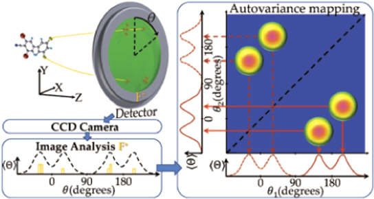
Figure 7. The principle of angle-resolved covariance mapping. A VMI spectrometer projects molecular ions from a Coulomb explosion onto a position-sensitive detector. The ion detection angles are recorded at each laser shot in the form of 1D spectra that are used to construct the simple covariance map (formula (3)) shown schematically in the right panel. The positions of the islands on the map reflect the molecular geometry. Reprinted with permission from [22]. Copyright 2012, AIP Publishing LLC.
Download figure:
Standard image High-resolution imageIn a further development of this technique the CCD camera is replaced by a multihit ultrafast sensor capable of 12.5 ns time resolution, albeit with only 72 × 72 pixel spatial resolution [23]. The high TOF resolution effectively separates the images according to the fragment masses (see figure 8, column I). This allows the authors to calculate selective covariance maps where, for example, only N+ ions are correlated with only F+ ions. The four-fold dimensionality is reduced to two dimensions by further processing. The angular position of the N+ ion is designated as the reference direction; the full, 4D map is rotated pixel-by-pixel to align the reference directions and the map is integrated over the radial N+ position. Such a procedure gives a type of recoil-frame covariance map (column II), in which the velocity vectors of the reference ions are confined along a single direction and the covariances with partner ions are shown relative to this direction. While the major molecular axis has been aligned with the spectrometer axis, the alignment of the planes of the two carbon rings is random. To remove this randomness an inverse Abel transformation is applied to the maps. The result displayed in column III shows a striking resemblance to the structure of the molecule depicted on the right. This technique is very promising for temporal monitoring and control of structural coordinates within polyatomic molecules, particularly concerning bond angles [24].

Figure 8. Advanced processing of angle-resolved covariance maps. Mass-selected fragment images (column I) are used to construct four-dimensional simple covariance maps held in computer memory. Rotating 2D segments of the 4D map aligns the ejection directions of the reference ions (here the N+ ions) giving recoil-frame covariance maps of F+ ions (row a) and Br+ ions (b). An inverse Abel transformation removes the cylindrical ambiguity of the experimental conditions (column III) and recovers the position of the fluorine and bromine atoms in the molecular structure shown on the right. Reprinted figure with permission from [23]. Copyright 2014 by the American Physical Society.
Download figure:
Standard image High-resolution image6. Gamma ray covariance maps
In nuclear physics covariance mapping has a distinct advantage over coincidence techniques in situations where data are heavily polluted by noise, or when data rates are so high that false coincidences obscure the true ones. Figure 9 shows 1D spectra and their simple covariance map for gamma rays registered by a pair of NaI detectors in a close proximity to a 60Co source masked by a stronger 22Na source [25]. On the 1D spectra three features from the 22Na decay are visible: a gamma peak at 1275 keV, a para-positronium annihilation peak at 511 keV, and a three-photon continuum from ortho-positronium annihilation at the lowest energy. The covariance map clearly reveals gamma cascades from the weak 60Co source (islands a and b), which on the 1D spectrum are masked by a strong 22Na cascade (c). Additionally, the continuum is resolved into a rich structure that involves Compton scattering and crosstalk between the detectors. In general, covariance maps provide much more distinctive fingerprints of radionuclides than 1D spectra.

Figure 9. An example of a gamma-ray simple covariance map. The map reveals a weak 60Co source (islands a and b) in the presence of a much stronger cascade from 22Na (c). Reprinted with permission from [25]. Copyright 2013, AIP Publishing LLC.
Download figure:
Standard image High-resolution imageThe Compton crosstalk between two detectors was employed to sense the directionality of gamma rays [26]. Figure 10 shows covariance maps of gamma rays from a 137Cs source registered by two NaI(Tl) detectors placed in close proximity on a turntable (see inset). When a 662 keV gamma ray emitted from the source undergoes Compton scattering in one of the detectors, the detector records the recoil electron, and the other detector records the scattered gamma ray. As the two detected particles share the original energy, their correlation forms a line on the map crossing the axes at 662 keV. Moreover, the energy sharing depends on the scattering angle (which is a consequence of energy and momentum conservation in the Compton process), so the maximum of the correlation line varies with the turntable angle as the left and right panels of figure 10 demonstrate. Calibrating the position of the crosstalk correlation, either theoretically or experimentally, gives a sensitive and quite inexpensive directional sensor of gamma rays.
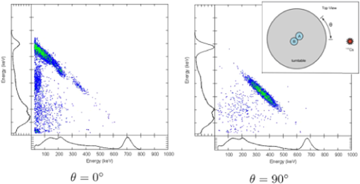
Figure 10. Directional gamma sensing using simple covariance mapping of Compton crosstalk. The crosstalk position on the map depends on the source-to-detector azimuthal angle θ (see inset). Reprinted with permission from [26]. Copyright 2014, AIP Publishing LLC.
Download figure:
Standard image High-resolution imageWhile coincidences can be employed in the construction of this sensor, the covariance technique offers greater flexibility of signal handling and better noise rejection. The latter is particularly important in this application because the crosstalk signal rides on a very large background of the direct signal.
7. Constraints and artefacts
While covariance mapping is an attractive technique, it has its limitations and characteristics that require attention at the planning stage of an experiment.
7.1. Signal-to-noise ratio (SNR)
To assess whether covariance mapping is suitable in a particular application it is helpful to estimate the SNR of the map using an example of a parent ion fragmenting into two daughter ions:

If the sample is dilute or the probability of such a fragmentation is low then the shot-to-shot number of fragmenting parent ions P follows the Poisson probability distribution with the mean value p:

However, the average number of detected daughter ions is usually lower due to imperfections in their detection:


where α and β (≤100%) are detection efficiencies that represent any particle losses on the way to the detector and the detector's quantum efficiency. Generally, the detected ions can be spread over several energy channels of the X and Y spectra. For the sake of clarity, however, we assume that they gather in two single but distinctive channels giving two peaks of amplitudes 〈A〉 and 〈B〉 on the 1D spectrum. Since the variance of a Poisson distribution is equal to its mean, the variance of the former peak after N laser shots is

and the SNR at this peak is
Deriving an equivalent formula for the (A, B) island on the covariance map is more laborious [27], since it requires calculating moments of bivariate Poisson distribution up to the 4th order. Following work [27] the results are1 :
The practical implications of equations (6) and (7) are discussed in the following sections.
7.2. Collection and detection efficiency
In experiments with particles it is essential to have high combined collection-detection efficiencies, since the SNR on the map given by equation (7) is proportional to  Ideally, all particles emerging from the interaction region should be collected by the detector(s). This means that conventional spectrometers with small acceptance angles, such as hemispherical or magnetic-sector ones are usually unsuitable, unless one works with collimated beams of particles. For example, if isotropically distributed particles are accepted only within a half-cone angle θ = 1°, then the detection efficiency β ≤ πθ2/4π ≈ 10−4 and the SNR on the map relative to the 1D spectrum given by the ratio of equations (7)–(6) is less than
  For charged particles emerging in all directions the most suitable spectrometers are magnetic bottle or VMI for electrons and TOF with a short drift tube for ions. Any grids or meshes should be avoided as they reduce the collection efficiency.
Electron detectors, such as microchannel plates or channeltrons, have high quantum efficiency, approaching α = 70%. However, the same detectors when used for ions have lower quantum efficiency, normally around 20%. While in principle this efficiency can be increased by applying a higher potential on the front of the detector so that the ions hit it with a higher velocity, in practice the required potential of tens of kilovolts is too cumbersome to use.
7.3. Event rate
The reader may wonder why low detection efficiency α cannot be counteracted in the same way as it is routinely done with 1D spectra, i.e. by increasing the sample density, which in turn increases the event rate p and brings the product pα to the optimal level in equation (6). Unfortunately, such a procedure fails for covariance mapping (and for coincidences) because there is another limit on the event rate that is absent in 1D measurements. This limit originates in the noise of the uncorrelated product that must be subtracted from the correlated one (see panel (a) less (b) giving (c) in figure 5). In equation (7) this noise is represented by the p(1 + αβ) term, which for p → ∞ limits the SNR on the map to

and defeats the attempt to compensate for low values of α and β. Moreover, as the event rate increases the subtraction of 〈Y〉〈X〉 from 〈YX〉 becomes sensitive to higher order effects because both these terms are proportional to the square of the event rate, while their difference only varies linearly with this rate.
One such secondary effect is the presence of any uninteresting, common-mode correlations, which can be suppressed using partial covariance mapping as described in section 3. While a calculation of the SNR for partial covariance awaits rigorous treatment (such as an extension of work [27]), some qualitative guidance can be derived from experimental practice. Partial covariance tolerates an event rate of about an order of magnitude higher than simple covariance mapping. Figure 11 shows some single-shot TOF spectra that were used to calculate the covariance maps in figures 3 and 4. Pulses from individual electrons are well separated at longer flight times, but they pile up at the main photoelectron line. Typically, partial covariance mapping can cope with up to 10 single-event pulses piling up before other effects (such as imperfect monitoring of I, non-Poissonian event statistics, detector or physical process nonlinearities, etc) render the process of subtraction in equation (5) deficient. Likewise, simple covariance mapping can typically accommodate only occasional pileup of two pulses, and coincidence techniques normally work with less than one event per spectrum, i.e. the majority of the spectra are empty.
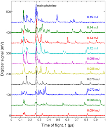
Figure 11. Examples of single-shot electron spectra for different x-ray pulse energies. Partial covariance mapping can accommodate several pulses piling up (mostly at the main photoline) and still give a clean map shown in figures 3 and 4. Reprinted from [15]. © 2013 American Physical Society.
Download figure:
Standard image High-resolution imageEven in the absence of adverse common-mode correlations, working with high pileups brings little improvement to SNR because it approaches the asymptotic limit (8) at high event rates. It may seem, therefore, that pileups of only a few pulses are sufficient. However, while such an event rate may be sufficient for the strongest peaks it would be too low for weak features, which are often the most interesting ones. Consequently, the event rate should be optimised for the strongest peaks of interest, allowing correlations with any stronger but uninteresting peaks to become distorted and accepting that for weaker peaks such an event rate is sub-optimal. In practice, the event rate is set by watching the single-shot spectra in real time and adjusting the pileups in the region of interest.
7.4. Number of shots required
The duration of an experiment is determined by the total number N of single-shot spectra needed and, as in any signal averaging, the SNR is proportional to  By knowing the detector efficiencies α and β, and specifying a certain level of SNR, N can be estimated from equation (8). For example, for typical α = β = 30% and SNR = 100, the required N is around 103. However, this assumes that there is no background of other islands overlapping island (A, B). A reasonable separation of features masked by a comparable background typically requires N ≈ 104, which translates to about ½ h of data collection at a 10 Hz repetition rate. If higher repetition rates are feasible, it is worth noting that for N > 105 the covariance map has such a large dynamic range that a linear colour scale becomes inadequate (see the nonlinear colour scale in figure 3).
7.5. Analog-to-digital converter (ADC) resolution
Normally, the analog signal from the detector is digitised by an ADC. Often the signal is a fast transient that requires a high-performance ADC with not only high sampling rate but also sufficiently high resolution of the signal level. The first requirement is that the signal noise should be resolved, because there may be a weak feature that is masked by the noise in any single shot but can be made visible upon averaging the noise over many shots. The averaging procedure works only if the noise fluctuations are resolved; around 2 bits of the ADC resolution are sufficient for this purpose. Secondly, the event pulses have to be resolved. These pulses are often of varying amplitude and some of them pile up. Typically, 6–8 bits of resolution are needed here.
In practice, an 8 bit ADC is normally sufficient for simple covariance mapping and a 10 bit ADC is needed for partial covariance mapping. It is worth noting that the required resolutions are the effective ones; they are notoriously lower than the advertised nominal ADC resolutions, especially at high sampling rates. The difference between the nominal and effective resolution is the internal ADC noise level, which may show on the map if the ADC specifications are not carefully scrutinized.
7.6. Detector saturation and converter clipping
Covariance mapping assumes that the arguments in the covariance formula closely follow the corresponding physical quantities. Any nonlinearity in the signal processing can generate artefacts on the map.
The most common source of nonlinearity is detector saturation. For example, a pulse from a microchannel plate detector depletes the charge in several neighbouring channels and renders them inactive for a while. If another particle hits the detector near the same place during this dead time, it will produce a smaller pulse or none at all. Sometimes this detector saturation cannot be avoided at strong peaks, producing spurious lines on the map. For TOF spectra the distortion may also affect features that occur at times later than the saturated peak, since microchannel plates usually require a few microseconds to recover.
Moderate deviations of the ADC scale from a linear function do not produce spurious features on the map because all signal samples are affected in the same way, which only slightly distorts the vertical scale of the whole map. A more drastic source of nonlinearity is signal clipping, i.e. when the signal exceeds the ADC range and the output is clipped to the minimum or maximum value. Any samples that are clipped more than once do not contribute to covariance, since cov(Y, X) = 0 if Y or X are constant, which effectively lowers those map features affected by clipping. While the distortion caused by clipping is not severe, it can be completely removed by rejecting clipped spectra.
7.7. Unbiased covariance estimators
Equation (3) gives slightly underestimated values for covariance. The result would be exact if the mean value of X was precisely known, but since the mean is estimated in equation (2) a degree of freedom has been used from N shots, so expression (3) should be multiplied by a factor of N/(N − 1) to give an unbiased estimate of covariance. Likewise, the partial covariance formula (5) uses another degree of freedom to estimate the correction, so the whole expression should be multiplied by N/(N − 2). Explicit formulae that include these factors are given in the supplemental material of [15].
7.8. Negative covariance
There is considerable confusion regarding interpreting regions of negative covariance. At first glance a negative island on a map suggests the presence of competing processes. However this interpretation is often unfounded and one should not jump to such conclusions before considering alternatives.
It may seem that the competition between fragmentation paths of a parent molecular ion, P, leading to different daughter ions, e.g.
can be revealed by measuring a negative covariance between either A or B with C or D. The reasoning is that if P leads to A then it does not lead to C, therefore ion pulses at A and C should be anticorrelated and cov(A, C) < 0. Unfortunately, such reasoning is flawed because P is not the same individual in both lines of equation (9). The two fragmentation paths can be taken only by two different individual ions:
If the sample is diluted, such as gas, there is no interaction between P1 and P2 (they have probably never even met). Therefore the two fragmentation paths are statistically independent, which should give cov(A, C) = 0 [28].
Yet, there is another complication. The above argument assumes that all single-shot spectra are recorded in identical conditions, which is only approximately true. Experimental conditions often fluctuate, inducing common-mode correlations (see section 3). In the presence of such fluctuations P1 and P2 can no longer be regarded as independent and it may happen that cov(A, C) < 0, for example, when the excursion of a fluctuating parameter enhances the A + B path at the expense of C + D.
It seems that laser intensity fluctuations may be responsible for negative covariance values measured in Coulomb explosion of ammonia [29] and pyridine [30] clusters. For example, low-intensity pulses produce mostly singly-charged large ammonia clusters, and high-intensity pulses tend to give multiply charged nitrogen ions, which gives negative covariance between the two species. Another possibility is that a jitter between molecular beam puffs and laser pulses effectively varies the cluster density or composition. Such jitter-induced fluctuation in sample composition is probably responsible for the negative line in figure 5(e). Negative covariance was also observed between peaks from laser-ablated ions [31, 32]. With such solid-state samples there are more possibilities to induce common-mode (anti) correlations, e.g. non-uniformity of sample composition, plasma instabilities or space-charge effects.
7.9. Initial map interpretation
When a structure gradually emerges from the noise during an experimental run, an immediate question arises: is it a real signature of the science we study or an instrumental artefact? Sometimes this question is hard to answer, but the following scrutiny is helpful.
Any structure that is qualitatively similar to the uncorrelated product, such as shown in figure 5(b), is likely to be an artefact due to some common-mode correlations. The easiest test of this possibility is to subtract a varying excess of the uncorrelated product and observe if the investigated structure is substantially suppressed for some value of the excess. Another test is to reduce the event rate by, for example, reducing the sample density, or attenuating the excitation if only linear processes are studied. Such a reduction of event rate suppresses common-mode correlations more than the direct ones, because the 〈Y〉〈X〉 term in equation (3) is proportional to the square of the event rate while the 〈YX〉 term is only linearly proportional to this rate, as discussed in section 7.3. Therefore, any structure that persists in the limit of low event rate provides evidence of direct correlations between two regions of the Y and X vectors.
When interpreting the map, one should keep in mind that the noise level is not uniform. Not only it is elevated on prominent islands, but is often also fairly strong on weak features. This is because the noise on the map is the sum of the noise levels of the correlated and uncorrelated products, so the map noise is always elevated whenever the sum is large, regardless of the difference of the mean levels. The noise variation makes the choice of colour scale quite important. For example, one should avoid colours that emphasise the positive noise excursions more than the negative ones, since such imbalance may create an illusion of an island being stronger than it is when only the noise is stronger. For the same reason, cutting off negative values often produces illusory features in noisy regions of the map.
7.10. Simulations
Covariance mapping experiments are straightforward to simulate. Matching the simulated maps to the experimental ones is often the easiest way to unravel the underlying physics. However, when writing the simulation code the programmer needs to keep in mind that covariance is sensitive to even small distortions in the random variable distributions. For example, in the gas-phase experiments, the number of sample species in the interaction region follows the Poisson distribution. Unfortunately, this distribution is awkward to handle numerically because of its infinite tail. Given finite computational resources, the usual solution is to cut off the end of the tail, but the cut-off needs to be quite high, so that in the whole simulation there is approximately only one event that exceeds the cut-off value.
8. Further advances and future directions
The covariance mapping technique is still being developed. This section outlines a personal view on the most promising research directions.
8.1. Coincidences versus covariance mapping
The recent growth of experimental implementations of coincidence and covariance mapping techniques has stimulated theoretical interest in this subject. A formal theory of noisy Poissonian processes with multiple outcomes has been developed [27] and used to compare coincidence and covariance schemes in simulated and real ionisation experiments where electrons and ions are detected with fractional efficiencies [33]. A detailed analysis of random and systematic errors allows the authors to find the optimal event rate, which for coincidence experiments is roughly 1 event per shot. At such a low rate, coincidence can outperform covariance only with highly efficient detectors. The authors show that with more typical, less efficient detectors, the covariance technique is a better choice, since in principle it can accommodate a much higher event rate, shortening an experiment's duration by orders of magnitude. The theoretical model allows for non-Poissonian (Gaussian) noise on the mean of the Poisson distribution. When experimental data are analysed, the authors demonstrate [33] that non-Poissonian fluctuations of sample density substantially distort covariance spectra. It would be interesting to extend this analysis to partial covariance mapping.
Another theoretical study [34] focuses on statistical analysis of coincidence experiments at high event rates, with the probability of more than one particle arriving at the same TOF no longer negligible (as was assumed in section 2.5). Starting from the simple covariance formula, the author derives a method for removing the background of false coincidences that are far beyond the limit of 1 event per shot. If this method works in practice, it may give coincidences an advantage over covariance at high repetition rates where the data flow from an ADC would be unmanageable.
8.2. 3D covariance mapping
The ability of covariance maps to reveal the parent species of two fragments invites the question of whether it is possible to do so for three fragments. Starting from the standard covariance expression (3), a three-dimensional (3D) extension of covariance was proposed [35]:
where indices i, j, k label three TOF samples. This expression was implemented in an experiment that uniquely identified the N2O6+ ion as the parent of three doubly charged daughter fragments.
In a more recent experiment [36] the 3D covariance map was used to analyse Coulomb explosion channels of carbonyl sulphide. The 3D covariance map is a volume map shown in figure 12. Since the map data are taken from a single detector, there is an autocorrelation line at the diagonal of the cube, x = y = z, and three autocorrelation planes: x = y, y = z or z = x. While the autocorrelation structures mask some information, the dark regions outside them pinpoint three-fragment correlations. The map enabled the authors to construct a hierarchical ionisation diagram of OCS, with two distinct energy groups and a few charge asymmetric channels that escape classical enhanced ionisation modelling.
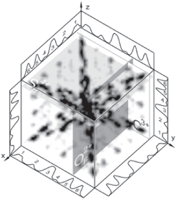
Figure 12. Three-dimensional covariance map of Coulomb explosion of a multiply ionised OCS molecule. The map allows one to uniquely identify Coulomb explosion channels involving three charged fragments. Reprinted figure with permission from [36]. Copyright 2006 by the American Physical Society.
Download figure:
Standard image High-resolution imageA theoretical analysis demonstrates that the 3D map values are proportional to the number of parent species if they follow Poissonian statistics, but not Gaussian [37]. Therefore, the 3D covariance mapping technique is most suitable for experiments in gas phase or where the excitation probability of any single species is very low.
8.3. 3D partial covariance mapping
The 3D covariance map given by equation (11) contains common-mode correlations induced by any fluctuating parameter I, as described in section 3. To remove such spurious correlations simple linear regression was used to model the X, Y and Z dependence on I, which led to a formula for 3D partial covariance [37]. The formula is rather long, involving several combinations of simple 2D and 3D covariances of the four random variables, but it is in a closed form and can be readily evaluated on a computer. The formula was tested in a simulated dissociative ionisation experiment, where 100% laser intensity fluctuations and on average 5 ionisations per laser shot were assumed. Figure 13 shows that intensity-induced correlations in the simple 3D map are removed when the partial covariance formula is used.
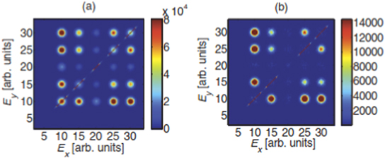
Figure 13. Simulated segments of a simple (a) and partial (b) 3D covariance map. In panel (a) laser intensity fluctuations induce spurious correlations, which are removed in panel (b). Reprinted figure with permission from [37]. Copyright 2014 by the American Physical Society.
Download figure:
Standard image High-resolution image8.4. 4D and higher dimensions
While the natural extension of equations (3)–(11) correctly captures the underlying physics, this heuristic recipe fails in 4 and higher dimensions [37]:
This failure could be illustrated by considering any two uncorrelated pairs of correlated random variables, such as Z correlated only with Y and X correlated only with W. This causes equation (12) to deviate from zero, whereas we require that non-zero values are obtained only when all variables are correlated with each other. Theoretical work [37] provides a rigorous proof of this property and shows that the values of expression (12) are no longer proportional to the number of parent ions that follow Poisson statistics. Devising correct formulae for multi-dimensional covariance of any degree higher than three is an open quest.
8.5. Multi-parameter partial covariance mapping
While publication [37] gives an analytical formula for partial covariance (2D) with two fluctuating parameters, it is quite easy to handle an arbitrary number K of such parameters numerically. If I is a row vector of K fluctuating parameters and IT is its transpose (a column vector), then the standard formalism of multivariate partial covariance [18] leads to:
where cov (IT, I)−1 is the inverse of the K by K dispersion matrix of parameters I and the backslash denotes the left matrix division operator, which bypasses the requirement to invert a matrix and is available in some computational packages such as Matlab. Since the units of I cancel out in the above equation, vector I may be composed of different physical quantities, such as laser pulse energy, pulse duration, sample density, etc, or they can be related, such as shot-to-shot samples of photon frequency spectra.
Although at this review's time of writing there are no published reports of using equation (13) to produce covariance maps, this multi-parameter technique seems to be particularly suitable for analysing data generated at FEL facilities, where the x-ray pulses are highly fluctuating but their spectral and temporal characteristic can be recorded at every shot. At these facilities a considerable technological development is directed towards producing increasingly shorter and more intense FEL pulses, while the scientific programme concentrates on understanding the physics of ultrafast interactions at a very high x-ray intensity. This concerted effort aims at implementing the 'diffract before destroy' concept to resolve the atomic structure of large biomolecules, viruses, and organelles (see [38] for a recent review).
8.6. Slicing
Equation (3) tells us first to calculate the averages over the whole data set, and then use them to calculate the covariance map. However, there is another way of producing the map, i.e. by dividing the data set into smaller slices, calculating the covariance map for each slice separately, and taking an average of these maps. The end result of the two procedures is similar but not exactly the same and slicing is often the better choice. For example, when there is a slow drift in experimental conditions, time slicing of the data set suppresses any common-mode correlations that are slower than the slice duration, effectively dropping the need to measure slowly-varying parameters and rendering the partial covariance formula unnecessary. When both slow and fast fluctuations are present, sliced partial covariance mapping can be used.
Slicing simplifies the display of partial covariance maps during data acquisition. As soon as enough data has been acquired for a slice, expression (13) can be executed and the map can be updated using the formula for the cumulative running average without the need to keep track of all covariance components separately.
The penalty for using slicing is that each slice consumes K + 1 degrees of freedom, where K is the number of fluctuating parameters in the partial covariance equation and K = 0 for simple covariance. This effectively reduces the number of shots in the whole data set by the number of slices multiplied by K + 1. Therefore, to avoid a significant deterioration of the SNR, the number of shots in a slice should be much larger than K + 1.
8.7. Contingent covariance
Contingent covariance mapping [37] is an advanced form of slicing that exploits other ways of grouping the data into slices, not just sequentially over time. For example, the data slices can be parameterised according to the excitation intensity (provided it is measured at each shot), or the slices can be multi-dimensional if several parameters are measured. In the same manner as for temporal slicing, covariance maps are calculated within each slice first and then averaged over all slices to give the final map that is contingent on parameter fluctuations not exceeding the slice width.
Contingent and partial covariance are alternative ways of suppressing common-mode correlations. The advantage of the former is that it does not assume linearity of these correlations, so it can be more effective in suppressing nonlinear effects such as multiphoton ionisation. However, contingent covariance consumes more degrees of freedom and is quite complicated to implement for online data monitoring.
In a recent experiment [39] a combination of partial and contingent covariance mapping was used to identify electron pairs associated with double core hole states created in acetylene and ethane by x-ray FEL pulses. The authors demonstrate that covariance mapping can reveal these states much more selectively than by using conventional 1D spectroscopy and requires about one order of magnitude less experimental time than coincidence techniques that use synchrotron radiation.
8.8. Stimulated Raman covariance mapping
Photon-photon covariance maps usually suffer from a high level of noise, since it is impossible to collect all photons if they are emitted in random directions. However, coherent processes such as stimulated Raman scattering (SRS) generate collimated beams of photons, which makes high collection efficiency possible. A promising application of covariance mapping to SRS spectroscopy of inner shell processes using x-ray FELs has been recently proposed [40].
While x-ray FEL pulses are sufficiently intense to induce SRS in inner shells, their wide bandwidth makes them unsuitable for spectroscopy at even a modest resolution. However, such pulses have much narrower substructure consisting of several fluctuating spikes formed in the process of self-amplified stimulated emission (SASE). The authors propose to apply covariance mapping to these fluctuations to improve the SRS FEL resolution by more than an order of magnitude.
Figure 14 shows the huge resolution improvement achieved in a simulated experiment. The stimulating pulse energy is centred on 867 eV and has a bandwidth of 7 eV, i.e. more than the vertical axis range. Correlations of these pulses with the scattered photon spectra (horizontal axis) reveal a series of Ne 1s−1np states, where n = 3–6. The resolution of the map is determined by the bandwidth of the spikes, which is about 0.1 eV corresponding to a 40 fs coherence length. It would be interesting to demonstrate experimentally that this technique does indeed make high resolution spectroscopy with SASE FELs possible.
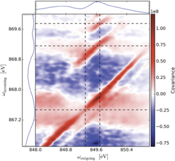
Figure 14. Simulated covariance map of x-ray stimulated Raman scattering in neon using fluctuating SASE pulses. The stimulating photon energy is on the vertical axis and the scattered photon energy is on the horizontal axis. The map reveals several core-excited levels of neon. These levels are unresolved on the conventional, 1D spectrum (top inset) because the bandwidth of the pulses is about twice the vertical axis range. Reprinted figure with permission from [40]. Copyright 2013 by the American Physical Society.
Download figure:
Standard image High-resolution image8.9. Connectomics
Covariance maps have been used to unravel brain connectivity by processing positron emission tomography (PET) images [41]. The images were averaged over two groups of 137 and 139 patients suffering from mild cognitive impairment related to Alzheimer's disease. In this study the meaning of 'map' is not the same in the previous sections: here it shows neural activity correlations mapped on the physical shape of human cerebral cortex, as shown figure 15. The correlations are with only one location on the cortex, called a 'seed', which is arrowed in the figure. In the context of this review these maps are segments of full covariance maps, which are four-dimensional if the cortex is considered to be a surface or six-dimensional if the cortical layers are resolved; the seeds of the full map form an autocorrelation surface or volume, respectively. However, since the map correlates only two brain locations, the 2D formula (3) is sufficient.

Figure 15. Seed-based covariance maps of human brain activity averaged over two groups of subjects (A and B) using positron emission tomography. The activity is relative to the seed region (arrowed), which corresponds to the autocorrelation line in figure 3. Figure reprinted from [41]. © 2014 SAGE Publications.
Download figure:
Standard image High-resolution image
The concept of partial correlation has been used in early PET studies of Alzheimer patients [42]. The partial correlation coefficient [43] is closely related to partial covariance; it is the partial covariance divided by the square roots of the partial variances of X and Y. The common-mode parameter in the evaluation of partial correlation [42] was the total PET signal, which was fluctuating significantly from individual to individual due to variability in the metabolism rate of glucose. The partial correlation maps were rather crude, correlating only 59 brain regions using a sample of 21 patients. It would be interesting to see if suppressing inter-individual fluctuations using the multi-parameter formula (13) could improve maps of brain activity.
Increasing the resolution and sensitivity of covariance mapping of PET and NMI scans is a potential route to untangling the wiring of the human brain. This research is relevant not only to brain disorders but also to an ancient philosophical problem: the relation between mind and body. In modern terms the problem is formulated as a search for neural correlates of consciousness [44]. One unexpected finding of such a correlate was the discovery of single neurons responding selectively to conscious recognition of famous people [45]. It is hypothesised that the phenomenon of consciousness itself is an emergent stochastic process of correlated neural activity [46, 47]. There are good prospects for testing this hypothesis using the technique of partial covariance mapping.
9. Concluding thoughts
A procedure that was conceived 30 years ago to study Coulomb explosion of molecules in picosecond laser pulses has grown into a general technique that is now used in many areas of science. The power of the technique comes from the use of two- and higher-dimensional statistical estimators to reveal causal relations hidden behind apparent randomness, thus giving it a significant advantage over one-dimensional techniques. Couple this with the benefit of modern computational technology (capable of increasingly faster processing of large data sets) and there is a plethora of new opportunities to apply both multi-dimensional and multi-parameter partial covariance mapping techniques not only within further fundamental research, but also to the development of a range of real life applications.
Acknowledgments
The author thanks the Engineering and Physical Sciences Research Council, UK for support (grants EP/F034601/1 and EP/I032517/1).
While this paper was in review, simple covariance mapping was used in x-ray FEL experiments to reveal the formation of double core holes in aminophenol [48] and to study the dynamics of Coulomb explosion of Ho3N@C80 molecules [49]. Femtosecond laser pulses in near IR were combined with 2D simple covariance mapping to study angular correlations of ionic fragments ejected in Coulomb explosion of diiodobenzene molecules, isolated or embedded in helium nanodroplets [50], and 3D simple covariance mapping was used to reveal the structure of 3,5-dibromo-3',5'-difluoro-4'-cyanobiphenyl molecules prior to their Coulomb explosion [51].
Footnotes
- 1
The detailed derivation for an electron–ion covariance map is in sections 2, 4 and 6 of [27]. To simplify the result, the histograms of ion mass and electron energy spectra have been reduced to single points by setting f(E) = f(M) = fM(M) = 1, the Gaussian noise on the mean of the Poisson distribution has been ignored by setting σ = 0, and the following variables have been renamed: NM → A, NE → B, ν0 → p, ξi → α, ξe → β, 1/Rstat → SNR.