

Abstract
We compare various theoretical approaches that are frequently used for modeling the excitation dynamics in photosynthetic light-harvesting complexes. As an example, we calculate the dynamics in the major light-harvesting complex from higher plants using the standard Redfield theory, the coherent modified Redfield theory combined with the generalized Förster theory, and the scaled hierarchical equation of motion (HEOM). The modified Redfield and coherent modified Redfield theories predict unrealistically fast transfers between weakly coupled and isoenergetic sites due to the secular character of these approaches. This shortcoming can be excluded by the artificial breaking of exciton mixing between these sites and invoking a generalized Förster theory to calculate the transfers between them. A critical cutoff indicating which exciton couplings should be broken is dependent on the energy gap between the corresponding sites (and therefore can be different for different parts of the complex). An adequate determination of the strongly coupled compartments of the whole complex allows us to obtain a quantitatively correct description with the combined Redfield–Förster approach, resulting in kinetics not much different from the exact HEOM solution.
Export citation and abstract BibTeX RIS
1. Introduction
The primary processes of photosynthesis occur in light-harvesting (antenna) complexes that absorb sunlight and transfer the excitation energy to the reaction centers (RC), where a charge separation is initiated [1–3]. The light-harvesting complexes are essentially heterogeneous, i.e. they are characterized by a big spread of pigment–pigment distances. They may contain monomeric pigments and tightly packed aggregates with strong excitonic interactions (dimers, trimers, etc). The excitation dynamics within strongly coupled clusters has the form of Redfield-type relaxation between delocalized exciton states, whereas intercluster migration resembles Förster-type hopping between weakly coupled compartments. In recent years, significant progress in our understanding of light harvesting in antenna complexes has been made using a theoretical approach where the modified Redfield model is combined with generalized Förster theory [4, 5]. The Redfield–Förster approach allows us to build a unified picture of the exciton structure and excitation dynamics in an antenna, where the linear and nonlinear (ps/fs) spectral responses can be modeled at a quantitative level after the structure-based exciton Hamiltonian and electron-phonon spectral density (extracted from experiment or calculated ab initio) are specified. Some of the parameters (like site energies that are difficult to calculate precisely) can be adjusted from an evolutionary-based search with a simultaneous fit of all the available spectra and kinetics. Such an approach has led to quantitative models of many antenna and core complexes, i.e. antenna complexes B800-850 [6], B800-820 [7], and B850 [8, 9] from purple bacteria, FMO complex from green bacteria [10, 11], PE545 complex from cryptophyte algae [12, 13], LHCSR3 complex from green algae [14], plant light-harvesting complexes LHCI (Lhca4) [15], LHCII [16, 17], CP29 [18, 19], core complexes of photosystem I (PSI) [4] and photosystem II (PSII) [20, 21], and the PSII reaction center (PSII-RC) [22–28].
Recently, a coherent modified Redfield (cmR) theory has been developed [29–31], containing transfers between the one-exciton populations together with the decay of the coherences. Unfortunately, nonsecular terms, i.e. transfers between coherences as well as transfers between populations and coherences, are not included. These terms are important to describe transfers between the weakly coupled and isoenergetic sites, where nonsecular transfers maintain long-lived coherences between the exciton (delocalized) eigenstates. These coherences keep the excitation localized, whereas in the secular approximation (where coherences quickly decay without being 'repumped' from the populations) initially localized excitations exhibit rather fast delocalization between the donor and acceptor states. In the site representation this looks like unrealistically fast energy transfer [32]. The cmR theory suffers from such a 'resonant artifact' similar to modified Redfield (where the coherences are not included at all). To circumvent it, the cmR can be combined with the generalized Förster theory, or with the small polaron quantum master equation [31]. In such combined approaches the most questionable point is how to determine the crossover between the two energy transfer regimes. The simplest way is to split the whole system into compartments, with the exciton couplings Mjj' exceeding some critical value, Mc [4, 5]. Then the dynamics within the clusters with Mjj' > Mc can be described with the Redfield theory, whereas the transfers between these clusters (with intercluster couplings Mjj' < Mc) are treated with the generalized Förster theory. The critical value Mc can be chosen intuitively [4, 5, 10, 16, 17, 20, 21, 33] or by comparing the results with those of exact methods, like the hierarchical equation of motion (HEOM) [32, 34–37].
Another limitation of the Redfield theory is connected with the positivity of the density matrix that generally cannot be guaranteed (depending on initial conditions, temperature, and details of the exciton–phonon coupling, like the correlation time etc) [38, 39]. This issue has been studied recently by comparing the Redfield (Bloch–Redfield) approaches to exact solutions [40, 41]. The problem has also been discussed in the context of the modeling of energy transfer in photosynthetic antenna complexes [42] and electron transfer reactions [43].
In this paper we calculate the excitation dynamics in the major light-harvesting complex LHCII from higher plants using the combined cmR-generalized Förster theory (cmRgF) and HEOM. In order to reduce the HEOM computing time we propose a simplified spectral density (in the form of a single overdamped Brownian oscillator) approximating a real spectral density and capable of reproducing the spectral profiles. In the cmRgF approach we split the complex into clusters, where the pigments j, j' within clusters are connected by strong couplings, i.e. Mjj' > Mc, implying that the biggest intercluster coupling is small, i.e. Mij < Mc. We show that such compartmentalization depends on the energy gap Eij between the most strongly coupled ith and jth sites from different clusters. If Eij is small enough we have to invoke the generalized Förster theory for intercluster transfers. In the case of a big gap Eij we can neglect nonsecular transfers and treat the intercluster dynamics with the modified Redfield theory, considering the two clusters as one (meaning that the new Mc' value is smaller than the former one Mc, because now Mij > Mc'). Comparing the cmRgF kinetics obtained for different compartmentalization schemes (with different Mc values) and the exact solution (HEOM) we show that the optimal Mc really depends on the energy gap between the sites, and therefore can be different for different parts of the complex. We demonstrate how to define a reliable cmRgF model using the LHCII complex as an example, and we propose that a similar approach can be taken for other photosynthetic antennae and core complexes. The thus defined cmRgF schemes allow a fine adjustment of the parameters of the exciton model (site energies, disorder values, etc) using an evolutionary-based search (with a quantitative fit of linear and nonlinear spectral responses), which is difficult to do with numerically expensive exact methods.
2. Model
The structure of the major light harvesting complex of higher plants (LHCII) is shown in figure 1. Each of the three subunits of the trimeric LHCII complex contains 14 chlorophylls (Chls) arranged in two layers. Analysis of the exciton couplings between the 14 Chls allows us to define several strongly coupled clusters within both the stromal- and lumenal-side layers (as shown in table 1). The arrangement of these clusters is shown in figure 2. One can expect the Redfield-type relaxation within strongly coupled clusters and the Förster-type migration between (weakly connected) clusters. The Förster theory also works in the case of large energy gaps, breaking the mixing of the donor and acceptor (even in the case of strong coupling between them). For example, in spite of the strong coupling between the Chls b and Chls a on the stromal side, they can be considered as separate clusters connected by Förster-type Chls b → a transfers.

Figure 1. Pigment–protein organization in the plant light-harvesting complex II (LHCII), viewing the whole trimer along the membrane from the stromal side (left) and viewing one monomeric subunit parallel to the membrane plane (right). The protein is shown in a ribbon-representation and the pigments as sticks. For clarity, the Chl phytyl chains and lipids are omitted. The separation between stromal- and lumenal-side Chls is indicated by a dashed line. The picture is produced using Protein Data Base, file 1RWT [44]. Colors: gray—protein; green—Chl a; blue—Chl b; yellow—lutein; orange—neoxanthin; magenta—violaxanthin or zeaxanthin.
Download figure:
Standard image High-resolution imageTable 1. Interaction energies Mjj' (cm−1) for a monomeric subunit of the trimeric LHCII complex calculated in the dipole–dipole approximation (data taken from [17]). The stromal- and luminal-side pigments are shown in separate blocks, each containing several groups of pigments corresponding to strongly coupled clusters. The biggest couplings are underlined and bold. Numbers within parentheses show the site energies (cm−1) based on our 77 K modeling [17] and adjusted from the fit of the room-temperature spectra. The site energies correspond to purely electronic transitions, i.e. do not include a reorganization energy shift. Notice that these energies correspond to the fit with a realistic spectral density. In calculations with a simplified single-component spectral density all the site energies should be further uniformly red-shifted by 120 cm−1 (see explanation in the text).
| a602 | a603 | a610 | a611 | a612 | b608 | b609 | b601 | a613 | a614 | a604 | b606 | b607 | b605 | |
|---|---|---|---|---|---|---|---|---|---|---|---|---|---|---|
| a602 (15117) | 0 | 38.1 | −11.3 | 9.6 | 15.8 | −5.8 | −19.2 | 49.6 | −4.9 | 0.6 | 6.4 | 5.6 | 7.1 | −0.7 |
| a603 (15247) | 38.1 | 0 | 12.9 | −2.7 | −0.7 | 6.7 | 96.6 | −5.8 | 2.6 | −6.7 | −3.2 | −8.8 | 1.2 | 1.1 |
| a610 (15033) | −11.3 | 12.9 | 0 | −24.9 | 23.1 | 61.9 | 3.8 | −5.9 | 7.2 | −1.5 | −4.1 | −3.2 | −0.1 | 1.6 |
| a611 (15075) | 9.6 | −2.7 | −24.9 | 0 | 126.9 | 4.3 | 4.3 | 24.8 | −6.1 | 4.5 | −3.8 | −2.5 | −2.7 | 1.3 |
| a612 (15057) | 15.8 | −0.7 | 23.1 | 126.9 | 0 | −1 | −2.5 | 9.1 | −0.4 | −0.1 | 4.6 | 3.1 | 3.0 | −2.8 |
| b608 (15633) | −5.8 | 6.7 | 61.9 | 4.3 | −1.0 | 0 | 36.0 | 2.7 | −2.0 | 1.3 | −2.7 | −4.9 | −4.4 | −5.1 |
| b609 (15591) | −19.2 | 96.6 | 3.8 | 4.3 | −2.5 | 36.0 | 0 | 3.7 | −2.9 | 2.3 | −7.2 | −0.1 | −11.9 | −0.7 |
| b601 (15759) | 49.6 | −5.8 | −5.9 | 24.8 | 9.1 | 2.7 | 3.7 | 0 | −10.7 | 3.5 | −2.5 | −1.8 | −2.4 | 0.7 |
| a613 (15135) | −4.9 | 2.6 | 7.2 | −6.1 | −0.4 | −2.0 | −2.9.6 | −10.7 | 0 | −50.2 | 2.1 | 1.4 | 2.2 | −1.4 |
| a614 (15224) | 0.6 | −6.7 | −1.5 | 4.5 | −0.1 | 1.3 | 2.3 | 3.5 | 50.2 | 0 | −3.4 | −2.1 | −3.2 | 0.3 |
| a604 (15420) | 6.4 | −3.2 | −4.1 | −3.8 | 4.6 | −2.7 | −7.2 | −2.5 | 2.1 | −3.4 | 0 | 104.5 | 35.9 | 3.3 |
| b606 (15721) | 5.6 | −8.8 | −3.2 | −2.5 | 3.1 | −4.9 | −0.1 | −1.8 | 1.4 | −2.1 | 104.5 | 0 | 59.3 | 29.7 |
| b607 (15582) | 7.1 | 1.2 | −0.1 | −2.7 | 3.0 | −4.4 | −11.9 | −2.4 | 2.2 | −3.2 | 35.9 | 59.3 | 0 | −4.4 |
| b605 (15549) | −0.7 | 1.1 | 1.6 | 1.3 | −2.8 | −5.1 | −0.7 | 0.7 | −1.4 | 0.3 | 3.3 | 29.7 | −4.4 | 0 |

Figure 2. Arrangement of Chls in LHCII. (left) Stromal-side layer of the LHCII trimer (each of the three monomeric subunits is encircled). Labeling of the pigments within a monomeric subunit is the same as in the original work of Liu et al [44]. Each of the three subunits are encircled. Chls are represented by three atoms: the central magnesium atom and two nitrogen atoms NB and ND (black) that for each Chl defines the direction of the Qy transition dipole. The stromal-side layer of each subunit contains strongly coupled clusters a610-611-612, a602-603, b608-609, and monomeric b601 that can be considered as a separate cluster or formally be included into the b601-608-609 cluster (see text). (right) Lumenal-side layer of the LHCII trimer. Arrangement of the pigments corresponds to the view from the stromal side (as in the left frame), but the stromal-side layer (which is above the lumenal one) is not shown. The luminal-side layer of each subunit contains strongly coupled clusters b607-b606-a604, a613-614, and the monomeric b605.
Download figure:
Standard image High-resolution imageNotice that partitioning into clusters (shown in table 1 and figure 2) is not unique. Below we analyze this scheme together with alternative ones by comparing the emerging Redfield–Förster pictures with the exact solution of the hierarchical equation of motion (HEOM) for the whole monomeric subunit.
3. Methods
In this paper we model the excitation dynamics in LHCII using different approaches, i.e. standard, modified, and coherent modified Redfield theories, the combined Redfield–Förster theory, and various versions of HEOM. The dynamics is determined by the spectral density of the system–bath (exciton–phonon) coupling that can be arbitrary in the Redfield (and Redfield–Förster) approach. In contrast, the HEOM method most often applies a simple spectral density in the form of an overdamped Brownian oscillator or a single underdamped vibration. Including just one more vibrational mode in the spectral density increases the number of equations immensely. Thus, using a complicated spectral density with 7–11 peaks (approximating the realistic shapes containing up to several dozen high frequency vibrations) requires powerful computing [36, 45]. In this section we define parameters of a simple spectral density (consisting of a single overdamped Brownian oscillator), that is still capable of describing quantitatively the spectral shapes and relaxation rates in LHCII at room temperature. The thus-defined spectral density can be used to compare the dynamics calculated with HEOM and various perturbative approaches.
A realistic spectral density for LHCII (based on measured low-temperature fluorescence line-narrowing profiles [46]) can be constructed as a sum of one low-frequency overdamped Brownian oscillator and 48 underdamped vibrations [47]. In figure 3 we use this spectral density to model the room-temperature absorption (OD) and fluorescence (FL) spectra of LHCII with the modified Redfield theory. We calculate the spectral profiles for one monomeric subunit, containing 14 Chls with the parameters listed in table 1. The site inhomogeneity value is σ = 90 cm−1. The inhomogeneity and phonon couplings are the same for Chls a and b.

Figure 3. Modeling of room temperature absorption (OD) and fluorescence (FL) spectra for LHCII. The measured data [48] is shown by points. Spectra calculated with the experimental spectral density consisting of an overdamped Brownian oscillator and 48 underdamped vibrations are shown by black lines. Grey lines show spectral profiles obtained with a spectral density in the form of a single overdamped Brownian oscillator. Inset shows the original spectral density with high-frequency vibrations (black) and a single Brownian oscillator (grey) in the 0–950 cm−1 frequency region.
Download figure:
Standard image High-resolution imageNow we switch from the realistic to a simpler spectral density consisting of a single overdamped Brownian oscillator. In order to reproduce the spectral profiles we need the characteristic frequency (damping constant) γj = 500 cm−1 and coupling (reorganization energy) of λj = 300 cm−1. The spectra calculated with this spectral density and using the modified Redfield theory are shown in figure 3. Obviously, the fit is not as good for such a simplified model. In particular, a single Brownian oscillator is not sufficient to reproduce the 740 nm FL sub-band determined by intense vibrations around 1200 cm−1. On the other hand, the FL profile in the region from 680 to 720 nm (corresponding to frequencies up to 800 cm−1) is reproduced well. Bearing in mind that the biggest exciton splittings in LHCII (corresponding to Chls b → a transfers) do not exceed 600 cm−1, we conclude that our simplified spectral density should give realistic rates for both intra- and inter-band transfers. Notice that the reorganization energy with such a spectral density (i.e. 300 cm−1 in the site representation) is less than the reorganization with the original spectral density (which is about 480 cm−1 due to the presence of intense high-frequency vibrations). To this end, all the site energies have been red-shifted by about 120 cm−1 (to compensate for the reduced reorganization shift of the exciton components) in order to reproduce the observed OD/FL peak positions (grey curve in figure 3). Below, we use this single-component spectral density and the shifted site energies in all the calculations performed both with the cmRgF and HEOM approaches. Using a simplified spectral density makes it possible to calculate the kinetics with HEOM with routinely available computational facilities.
In all numerical examples (presented in the following sections) we use the scaled hierarchical equation of motion developed by Zhu et al [49]. The main equations are given in appendix
Notice that quantitatively the same kinetics can be obtained with the original (nonscaled) HEOM, but in this case bigger cutoff values are required, i.e. Nc = 7–10. We have found that the original version of HEOM with the lowest-order temperature correction [50] gives the same results as the scaled HEOM with K = 0, whereas the original HEOM in the high temperature limit [51] gives sizable deviations (which can be expected, because our damping constant significantly exceeds the room temperature thermal energy).
Below we compare the HEOM solution with various versions of the Redfield theory (including combined Redfield–Förster approaches). It should be noted that we did not find any violation of the positivity of the density matrix in our numerical examples, where we have checked various initial conditions and various system–bath correlation times (by changing the damping constant γj).
4. Results
4.1. Equilibration within the stromal-side Chls a (N = 5 model)
As a first example we consider the dynamics within the two stromal-side Chls a clusters, i.e. a602-603 and a610-611-612 upon excitation of the blue-most a603 site (figure 4). We use the spectral density in the form of a single overdamped Brownian oscillator with γj = 500 cm−1 and various reorganization energies, i.e. λj = 10, 30, 100 and 300 cm−1. The population dynamics is calculated for one realization of the disorder (with the unperturbed site energies from table 1). For each reorganization energy value we compare site populations calculated with four theories, i.e. standard Redfield (sR) with the full relaxation tensor, coherent modified Redfield theory (cmR) in the Markovian (time-independent) limit (see appendix
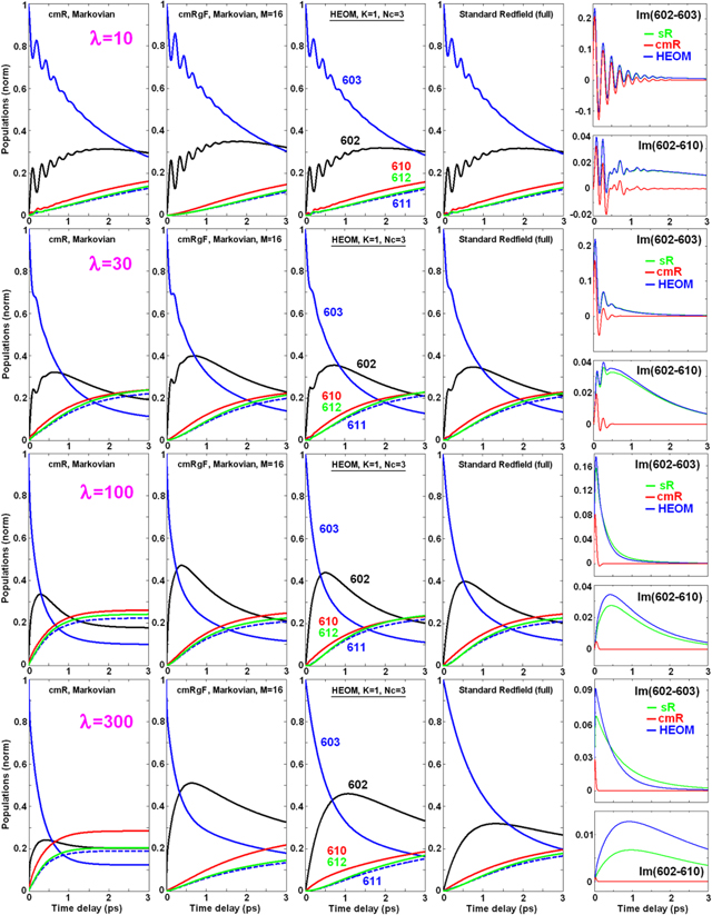
Figure 4. Population dynamics for the N = 5 model (including five stromal-side Chls a, i.e. a602-603-610-611-612) with an initially excited blue-most a603 site. Coupling to phonons: γj = 500 cm−1; λj = 10, 30, 100 and 300 cm−1 (from the top to the bottom rows). The calculation is done for one realization of the disorder (with the unperturbed site energies from table 1). Populations of the five sites in the 3 ps window are calculated with four different theories, i.e. sR, cmR, scaled HEOM (exact method) and cmRgF (with Mc = 16 cm−1, corresponding to the breaking of the coherent mixing between the a602-603 and a610-611-612 clusters). The two additional frames on the right side in each row show the imaginary parts of the coherences between the sites a602-603, and a602-610 calculated with sR (green), cmR (red) and HEOM (blue) (in the top frames the green curve coincides with the blue one). Notice that we do not include cmRgF coherences because the inter-cluster coherence (a602-610) disappears in cmRgF (where the inter-cluster transfers are described by the Förster theory), whereas the intra-cluster coherence (a602-603) is similar to the case of cmR.
Download figure:
Standard image High-resolution imageAt weak coupling to phonons (λj = 10 cm−1) all theories give almost identical kinetics with long-lived oscillations due to coherences between the a602 and a603 sites, and non-oscillatory a602-610 coherence due to nonsecular transfers. Notice that this non-oscillatory component is not present in the a602-610 coherence calculated with the cmR (which is a secular theory), as shown in the right frame of the top row of figure 4. Increasing the phonon coupling to λj = 30 cm−1 results in faster equilibration superimposed with damped oscillations. Again, the four theories predict very similar kinetics within an accuracy of some small differences. A further increase in coupling (to λj = 100 cm−1) produces even faster equilibration with non-oscillatory decay of the coherences.
Most interesting in the example shown in figure 4 is the dynamics of transfers between the weakly coupled (Mjj' < 15.8 cm−1) a602-603 and a610-611-612 clusters. Weak coupling implies intense nonsecular transfers that maintain the long-lived non-oscillatory coherences (like a602-610 and a603-610 coherences). Remember that the imaginary part of the inter-site coherences determines the coherences between the exciton eigenstates, that produce the exciton wavepacket localized at certain sites [32]. The breaking of these coherences produces exciton delocalization over the sites involved in the eigenstates. In this way the nonsecular transfers keep excitation localization on a602 and a603 sites, thus producing a relatively slow non-oscillatory population of the a610-611-612 sites. But in the secular theory the a602-610 and a603-610 coherences quickly decay (within 100 fs at λj = 100 cm−1 and even faster for bigger couplings) thus producing quick delocalization between the a602-603 and a610-611-612 clusters. As a result, the secular cmR predicts that the population of the a610-611-612 sites is too fast (see left frames in figure 4). After we artificially break the coherent mixing between the a602-603 and a610-611-612 clusters (invoking the cmRgF approach with Mc > 15.8 cm−1) the kinetics of a610-611-612 population becomes more realistic, i.e. not much different from the kinetics given by nonsecular approaches, i.e. sR and HEOM (see the third row in figure 4).
When increasing the coupling to λj = 300 cm−1 the secular kinetics is even faster than in the λj = 100 cm−1 case, whereas the cmRgF (as well as nonsecular sR and HEOM approaches) give slower kinetics. Comparing the kinetics at various couplings we conclude that they become gradually faster when increasing the phonon coupling (that is equal to the reorganization energy) from λj = 10 to 30 and 100 cm−1, but further increasing it to λj = 300 cm−1 starts to slow down the kinetics (except the secular ones). This is connected with an increase in the gap between the exciton states predominantly localized at a611-612 and at the red-most a610 site (due to an increase in the reorganization-induced shift of the lowest state localized at a610). This is mirrored by a pronounced increase in the steady-state population of the a610 site at λj = 300 cm−1 (that can be seen in the cmR kinetics in figure 4). The observed phenomenon reflects a general rule of the electronic energy transfers: more phonons produce faster transfers, but too many phonons make excitations less mobile due to reorganization-induced red-shifting, dynamic localization and self-trapping (polaron effects). Notice that the first factor is included both in the Redfield and HEOM, the second one (dynamic localization) is present only in HEOM, and the third factor (polaron formation) is not included in the HEOM (see explanation of these terms in appendix
It is also interesting to note that the equilibration rates are very similar in cmRgF, HEOM and sR when reorganization is not too big (λj < 100 cm−1). But for a realistic reorganization value of λj = 300 cm−1 the cmRgF approach gives faster kinetics (probably due to the instantaneous character of the bath relaxation caused by the Markov approximation both in the Redfield and Förster frameworks [51], whereas sR predicts slower kinetics (most probably due to its restriction to the weak coupling limit, implying a one-phonon character of exciton relaxation). Notice also that in cmRgF kinetics there is a very fast component in the a602 and a603 kinetics (<50 fs, with an amplitude of about 20%) connected with a quick decay of the a602-603 coherences (a feature that is not present in sR or HEOM, where coherences are more long-lived due to nonsecular transfers).
Alternative versions of cmRgF, where we break more exciton couplings, do not improve the results. Thus, we tried cmRgF with Mc = 25 cm−1, corresponding to breaking the coherent mixing between the a610 and a611-612 sites. This gives a localized (and more red-shifted) a610 site, which becomes more populated (compared with the a611-612 sites) in contrast with the true (HEOM) kinetics (data not shown). The cmRgF with Mc = 25 cm−1 is therefore not as good as with Mc = 16 cm−1. We thus conclude that breaking the couplings between 16 and 25 cm−1 is not justified.
The equilibration dynamics within the whole stromal side layer (containing five Chls a and three Chls b) can be satisfactorily modeled with the same critical coupling, i.e. Mc = 16 cm−1, as shown in figure S1, which is available at stacks.iop.org/JPB/50/124003/mmedia (see supplementary data).
4.2. Chls b → Chls a transfers in the luminal side (N = 6 model)
Now we switch to excitation dynamics at the luminal side. Here the a613-614 dimer is very weakly (2–3 cm−1) coupled to the a604-b605-606-607 compartment. Due to weak coupling in combination with a big energy gap between the a613-614 and a604-b605-606-607 sites (the nearest in energy a604 and a614 sites are separated by 204 cm−1 (see table 1)) we consider them as different clusters. We should also consider b605 separately from the a604-b606-607 sites (as will be justified below), meaning that the luminal-side pigments are split into three clusters, i.e. a613-614, b605 and a604-b606-607, corresponding to cmRgF approach with Mc = 30 cm−1.
Initial coherent excitation of the b606-607 dimer is followed by the population of the b605 and a604 bottleneck sites with subsequent very slow (30 ps) population of the a613-614 dimer. Kinetics are the same at very weak coupling to phonons (λj = 10 cm−1), but a slight increase in coupling to λj = 30 cm−1 reveals a pronounced difference between secular (cmR) and nonsecular approaches (figure 5). Thus, the b605 population is much faster in cmR. To explain this phenomenon we note that the b605 site is in resonance with the lowest exciton level of the b606-607 dimer (predominantly localized at b607). In such a situation the transfers between the b605 and b607 sites are very sensitive to inter-site coherences. Thus, a long-lived imaginary part of the b605-b607 coherence will maintain the localization of the excitation at the initially excited b607 site and prevent quick population of the b605 site (as revealed by HEOM and sR dynamics). But in the secular approximation (in cmR) a quick decay of the b605-b607 coherence (due to the absence of nonsecular coherence transfers) produces fast delocalization with equilibration of the b605 and b607 site populations. Such a difference between the cmR and HEOM/sR kinetics becomes even more dramatic at a realistic coupling value (λj = 300 cm−1), when the b605 and b607 populations are almost equal after 100 fs (within the cmR picture) in contrast with the nonsecular dynamics (HEOM, sR) giving slow (ps) equilibration between b605 and b607. This artifact of the cmR theory can be corrected by switching to the cmRgF approach, i.e. by considering the b605 and a604-b606-607 as separate clusters. Breaking the mixing of b605 with the b606-607 sites in cmRgF (meaning that Mc = 30 cm−1) gives a result that is very close to the exact solution (HEOM).
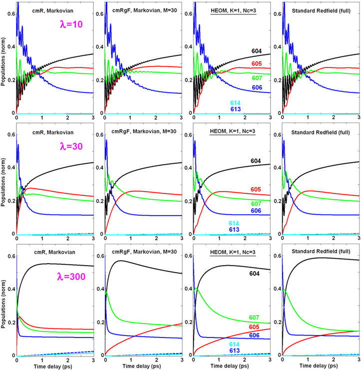
Figure 5. Population dynamics for the N = 6 model (including all the lumenal–side pigments, i.e. a613-614, a604 and b605-606-607) with initial coherent excitation of the b606-607 dimer. Coupling to phonons: γj = 500 cm−1; λj = 10 (top), 30 (middle), and 300 cm−1 (bottom). The calculation is done for one realization of the disorder (with the unperturbed site energies from table 1). Populations of the six sites in the 3 ps window are calculated with four different theories, i.e. sR, cmR, HEOM (exact method), and cmRgF (with Mc = 30 cm−1, i.e. considering b605 and a604-b606-607 as separate clusters, and with a613-614 as a separate cluster).
Download figure:
Standard image High-resolution image4.3. Equilibration within the whole subunit (N = 14 model)
Finally, we calculate the dynamics within the whole monomeric subunit of LHCII containing 14 Chls. The initial conditions are the same as those that we used in calculating the kinetics within the stromal- and luminal-side layers, i.e. we suppose broad-band excitation of all the Chls b (except red-shifted b605), including initial coherences within the b606-607 and b608-609 dimers.
Couplings between the stromal-side and luminal-side pigments are quite small (Mjj' < 12 cm−1, see table 1), so the transfers between the exciton states from different layers should be calculated using the generalized Förster theory, because the modified Redfield theory can give strongly overestimated rates in this case. To check this we compare the population dynamics calculated with the cmR theory (see figure 6) with the cmRgF approach with Mc = 12 cm−1, considering the stromal-side and luminal-side layers as two separate clusters, while retaining all the exciton interactions within these clusters, and, therefore, treating the dynamics within each layer with the modified Redfield theory (in figure 6 we denote this two-cluster model as cmRgF-2). In the cmRgF picture we have slow transfers from the a604-b605-606-607 sites to the a613-614 dimer on the luminal side. The a613-614 sites are also getting populated due to transfers from the stromal-side a602-603 sites. When we switch to the cmR picture and include exciton mixing between the layers, we find much faster transfers, including (i) a quick (sub-ps) rise of the a613-614 population due to transfers from a602-603 (see their reduced populations on the sub-ps scale), and (ii) faster decay of the a604-b605-606-607 populations due to transfers to the stromal-side pigments. Obviously, these fast transfers are artifacts of the modified Redfield theory, appearing when considering migration between weakly coupled and quasi-resonant sites [5]. These artifacts are connected with the secular character of the modified Redfield model [32].

Figure 6. Population dynamics in the whole monomeric subunit of LHCII (containing N = 14 molecules) with initial excitation of the Chls b, including b601, b606-607 and b608-609 dimers. Coupling to phonons: γj = 500 cm−1; λj = 300 cm−1. The calculation is done for one realization of the disorder (with the unperturbed site energies from table 1). Populations are calculated with the sR, cmR, HEOM (exact method), cmRgF-2 (with Mc = 12 cm−1, giving two clusters) and cmRgF-6 (with Mc = 16 and 30 cm−1 for stromal and luminal sides, respectively, giving six clusters).
Download figure:
Standard image High-resolution image
The two-cluster cmRgF-2 model gives a more correct description of the transfers between the two layers, but in order to obtain a more realistic picture of the dynamics within stromal- and luminal-side layers we have to split each of these layers into several separate clusters. As suggested in previous sections, realistic dynamics can be obtained by considering three clusters in the stromal side, i.e. a602-603, a610-611-612 and b601-608-609, and three clusters in the luminal side, i.e. a613-614, a604-b606-607 and b605. Altogether, we have a six-cluster model (denoted as cmRgF-6 in figure 6).
The main differences between the cmRgF-2 and cmRgF-6 models are related to (i) slower transfers from a602-603 to a610-611-612, and (ii) slower population of b605 in the cmRgF-6 picture (the same features have been observed in cmRgF models for the separate layers, as shown in figures 4, 5 and S1). Notice that the cmRgF-6 model is closer to the exact HEOM solution. The most remarkable differences between these two models become apparent as (i) a bigger population of the b607 site at sub-ps delays and (ii) non-monotonous kinetics of the a610 population (with a fast component on the 0.5 ps time scale) in the HEOM picture. Notice that similar features are also present in the sR model (at least within the 0.5 ps time window), so that they can be assigned to nonsecular transfers. Another factor that can influence the HEOM kinetics is the non-Markovian character of the off-diagonal phonon-induced fluctuations, that determine the (time-dependent) relaxation dynamics and a shifting of the exciton eigenstates (features not included in the standard and modified Redfield pictures). This may be the reason for the deviation of the a610 kinetics in HEOM from both sR and cmRgF models. In spite of these discrepancies the cmRgF-6 model looks very realistic. Notice that the sR approach gives the same character of the dynamics but the transfers corresponding to big energy gaps are too slow (most probably due to the one-phonon character of relaxation in the sR restricted to weak exciton–phonon coupling). Thus, the b → a transfers on the stromal side (corresponding to the biggest gaps) are most difficult to explain with the sR theory (see the dynamics of b601-608-609 depopulation in figures 6 and S1).
Notice that the damping constant (γj = 500 cm−1) used in all our examples (figures 4–6) corresponds to fast dephasing (about 10 fs), meaning that the dynamics is close to the Markovian limit. In this respect, it is interesting to study the relation between the Markovian cmRgF model and the exact HEOM solution also for other damping constants γj, especially for the reduced γj values corresponding to, essentially, a non-Markovian regime. Modeling of the kinetics with tuning γj from 100 to 800 cm−1 has shown (see supplementary data, figures S2 and S3) that in spite of some deviations from HEOM, the cmRgF-6 model is still capable of reproducing the equilibration within the whole monomeric subunit even at low values of γj. Notice, in this respect, that in real photosynthetic antennae the spectral density typically contains intense vibrations with the frequencies up to 1700 cm−1 [46, 47]. Therefore, modeling of energy transfers with a low-frequency spectral density (for example, with γj = 100 cm−1) is not realistic. On the other hand, the model with γj = 500–800 cm−1 gives a better approximation of the spectral density and the spectral lineshapes (as shown in figure 3). So, we believe that our choice of an overdamped Brownian oscillator with γj = 500 cm−1 yields a reasonable picture of the dynamics.
Comparing the kinetics calculated with cmRgF and HEOM, one should bear in mind that the observed differences can be determined by two factors. Firstly, the transfer rates (connecting the same pair of eigenstates) can be different when evaluated exactly or perturbatively. Secondly, the properties of eigenstates (like delocalization, phonon-induced shift, homogeneous broadening) are also different if they are treated by different approaches. These properties manifest themselves in linear spectral responses, for instance, in absorption lineshapes. In the modified Redfield model the absorption spectrum is calculated by explicitly including the diagonal exciton–phonon coupling [52], whereas off-diagonal coupling is given by a phenomenological Markovian term determined by the inverse lifetime of the exciton states (the thus-defined term is real and describes a relaxation-induced broadening) [12, 32]. In recent papers more versatile theories of absorption lineshapes have been developed [53–56], containing nonsecular and non-Markovian generalizations of the modified Redfield lineshapes. In section S3 of the supplementary data we have studied the absorption spectra of LHCII, calculated with modified Redfield theory, complex time-dependent Redfield (ctR) theory [54], and HEOM. We conclude that both ctR and HEOM give significant and nonuniform red-shifting of the exciton transitions (as compared to the modified Redfield theory). As a result, the relative energies of the exciton states are different in the cmRgF and HEOM models. This factor is responsible for the differences in kinetics shown in figure 6 (together with other factors connected with different treatment of the phonon-induced transfers between the states in cmRgF and HEOM).
5. Discussion
5.1. The choice of critical coupling
The modified Redfield approach should be replaced by the Förster theory for transfers between sites that are (i) weakly coupled and (ii) separated by a small energy gap Ejj'. In the case of big gaps the exciton mixing is not significant (being proportional to the Mjj'/Ejj' ratio that for large gaps is small both for weak and strong exciton coupling Mjj'). It means that the Förster theory can be applied, but the modified Redfield approach will work in this case as well, because nonsecular interactions are not important in the case of large gaps [32]. So, in order to define a suitable compartmentalization scheme we have to check all the sites with a relatively small energy difference Ejj' (compared to the static disorder value) and order them in the form of blocks with the weak (Mjj' < Mc) couplings between the sites from different blocks. The optimal value of Mc can be dependent on the gaps Ejj' and the details of the pigment mixing within these blocks. To find this optimal value it is useful to compare the exact solution (HEOM) with the Redfield–Förster kinetics for schemes with various Mc (switching from the lowest to larger Mc values, i.e. breaking in consecutive order more and more exciton couplings). A realistic Redfield–Förster picture can be achieved with different Mc values within different parts of the whole complex. Thus, in our best six-cluster model for LHCII Mc = 16 and 30 cm−1 for the stromal and lumenal sides, respectively. Such a comparison with HEOM (on finding an optimal subdivision of the whole complex) should be done at least for one realization of the disorder (for example, with unperturbed site energies). Then the thus built Redfield–Förster scheme can be used to adjust the parameters of the model via fitting of the available data using genetic algorithms (including averaging over disorder).
5.2. Comparing with other models of LHCII
It is remarkable that the Redfield–Förster picture developed in the present study (using the exact solution as a trial) is in agreement with previous models based on the fit of the spectral responses.
A consistent model capable of explaining the linear and fs pump–probe spectra for the LHCII trimer has been developed by Renger et al [16] using the modified Redfield–generalized Förster (mRgF) picture with the Mc = 20 cm−1 cutoff value. The spectral density included low-frequency phonons, whereas coupling to high-frequency intramoleculear vibrations was neglected. Such an approach allowed a semi-quantitative fit of the pump–probe kinetics [16]. A similar mRgF model with Mc = 15 cm−1 and with a realistic spectral density (the same as shown in figure 3, i.e. with 48 high-frequency vibrations) allowed a better quantitative fit of the linear spectra and pump–probe kinetics for different excitation wavelengths [17]. Notice that the model with Mc = 15 cm−1 gives overestimated rates of equilibration between the a602-603 and a610-611-612 clusters, as well as too fast population of the b605 site, according to the present study (see figure 6). But the exciton levels of the a602-603 and a610-611-612 clusters are well overlapped, so that the details of isoenergetic transfers between them do not significantly perturb the isotropic pump–probe kinetics on the red side of the absorption band. Similarly, the exchange between the b606-607 and b605 levels cannot be viewed in the kinetics. Obviously, such a scheme will not be sufficient to model the anisotropic pump–probe spectra, and to this end should be improved by switching to the more realistic mRgF (or cmRgF) picture with Mc = 16 and 30 cm−1 for the stromal- and luminal-side Chls (as shown in figure 6).
Recently, the population kinetics in the monomeric subunit of LHCII have been modeled with the HEOM and two versions of the mRgF, i.e. with Mc = 20 and 30 cm−1 [36]. Various spectral densities (approximating the experimental profile) have been used in this study, i.e. spectral densities containing three or seven vibrational peaks, and containing a single Brownian oscillator with a reorganization energy of λj = 220 cm−1. Remarkably, all the three spectral densities gave very similar kinetics (with an accuracy of weak oscillatory features present in the kinetics calculated with the 3,7-peak spectral density). The authors concluded that using a continuum of phonon modes provides a good description of the dynamics. It was also concluded that the model with Mc = 30 cm−1 gives better agreement with HEOM, especially for the b605 population (very similar to our results as shown in figure 6).
5.3. Comparing with models of other photosynthetic complexes
The Redfield–Förster approach has also been used to model the dynamics in other light-harvesting complexes from higher plants. Thus, modeling of the PSII core complex (including CP43, CP47 and PSII-RC subunits) was done using the mRgF with Mc = 36 cm−1 [20] and Mc = 30 cm−1 [21]. Notice that these models are restricted to a low-frequency spectral density with a reorganization energy of about 40–50 cm−1 (i.e. one order of magnitude smaller than the total reorganization including contributions from high-frequency vibrations). The same spectral density was used in the modeling of the whole PSII supercomplex (including LHCII, CP29, CP24 complexes and the PSII-core) that was done with HEOM and mRgF with Mc = 15 cm−1 [37]. It was found that the Mc = 15 cm−1 cutoff gives dynamics that are too fast compared with exact HEOM kinetics.
The Redfield–Förster theory was successfully used in the modeling of isolated PSII-RC [22–28]. To correctly reproduce the spectra and energy/electron transfer dynamics, a realistic spectral density (with reorganization of about 500 cm−1) is needed [24–28]. Different spectral densities have been compared by Gelzinis et al [27]. The exciton couplings between the six core pigments exceed 36 cm−1 [23], corresponding to the Redfield-type energy transfers. Transfers from the two peripheral Chls z (very weakly coupled (4 cm−1) to the six co-factors) correspond to the Förster limit. Transfers between the exciton and localized charge-transfer states (CT) should be modeled with the generalized Förster theory [25]. Notice, however, that the primary CT state can be mixed with the excited state of the primary donor due to the involvement of resonant vibrations. Such mixing cannot be described in a pure exciton basis, i.e. modified Redfield as well as Förster theories do not work in this case. The dynamics of the initial charge separation in the presence of electron-vibrational resonance can be described using the Redfield theory in the exciton-vibrational basis [57]. A resonance with quantized vibrations is also important in energy transfers in the antenna, as was demonstrated for the PE545 antenna complex [58] using the polaron master equation [59–61], and for the FMO antenna using HEOM [45].
A nice example of a complex with both strong and weak exciton couplings is the bacterial B800-850 antenna. The complex consists of two high-symmetry rings, i.e. the B850 ring containing 16–18 tightly packed and strongly coupled (250–300 cm−1) bacteriochlorophylls (BChl), and the B800 ring with 8–9 weakly coupled (about 20 cm−1) BChls. Experimental and theoretical studies have demonstrated the presence of coherent effects in the B800 antenna, that should be modeled with the Redfield theory [6, 7, 32]. Thus, the cutoff value can be estimated as Mc < 20 cm−1. Transfers from the B800 to the B850 ring can be described both by the generalized Förster [7] or by the Redfield theory [6] (due to the big energy gap, the results are the same). The isoenergetic transfers between neighboring B850 rings should be described by the generalized Förster theory, giving the same results as HEOM [34]. The generalized Förster and HEOM approaches also coincide in the case of LH2(B850)-LH1(B875) transfers [35].
6. Conclusions
We demonstrate the applicability of the Redfield–Förster approach for the modeling of energy transfers in photosynthetic light-harvesting complexes. An adequate determination of strongly coupled compartments of the whole complex allows a quantitatively correct description of the kinetics, free from the artifacts of the pure modified Redfield theory (mostly connected with its secular character). Neglecting nonsecular transfers can give a significant overestimation of the transfer rates between weakly coupled and isoenergetic sites. To avoid this artifact we have to artificially break the exciton mixing of these weakly coupled pigments and invoke the generalized Förster theory to calculate the transfer between them. Such an approach results in a more realistic picture that is not much different from the exact solution. A critical cutoff Mc, indicating which exciton couplings should be broken, is dependent on the energy gap between the corresponding sites. Thus, our modeling of the monomeric LHCII subunit demonstrates that a formal comparison of the exciton couplings Mjj' with some fixed Mc value is not sufficient to define a suitable (optimal) compartmentalization scheme.
Acknowledgments
VIN was supported by the Russian Foundation for Basic Research (Grant No. 15-04-02136); RvG was supported by the VU University Amsterdam, the Laserlab-Europe Consortium, the TOP grant (700.58.305) from the Foundation of Chemical Sciences part of NWO, the advanced investigator grant (267333, PHOTPROT) from the European Research Council, and by the EU FP7 project PAPETS (GA 323901), and by his Academy Professor grant from the Netherlands Royal Academy of Sciences (KNAW).
Appendix A.: Scaled hierarchical equation with low-temperature corrections
We consider the molecular aggregate made of N coupled pigments. The one-exciton Hamiltonian in the site representation is:
where  is the energy of the Frank–Condon transition (including the zero-phonon energy
  and reorganization energy λj), Mjj' is the interaction energy between the jth and j'th sites (the ωj0 and Mjj' values are listed in table 1). A coupling of the jth site to fast nuclear modes is described by the spectral density in the form of an overdamped Brownian oscillator (with reorganization energy λj and damping constant γj):
The scaled hierarchical equation of motion (HEOM) for the reduced density operator is [49]:
where σn denote auxiliary operators dependent on the set of integers describing the state of the phonon bath of the sites from j = 1 to N; n = {n10,..n1K,..njk,..nN0,..nNK};  the index k numbers the low-temperature correction terms from k = 0 to K; θ = kBT, where kB is the Boltzmann constant, T is the temperature. The auxiliary operators σn at n = {0,0,...0} are equal to the reduced density operator ρ. Here V×σ denotes a commutator, i.e. V×σ = Vσ − σV, where Vj = ∣j〉〈j∣. Notice that equation (A.3) implies that the phonons associated with different sites are uncorrelated. The dynamics of the one-exciton populations σii and coherences σij (in the site representation) is given by:
with ωij = ωi0 − ωj0., and with some initial conditions for σij describing the state of the system after impulsive excitation. For example, excitation of the jth site corresponds to  for n = {0,0,...0} and
  for other n sets. If the sum of njk exceeds Nc, then the terms with G, Gik, and Lik in equations (A.3) and (A.4) are set to zero [62]. The depth of the hierarchy Nc and the number of the Matsubara frequencies K should be chosen in order to get converging results.
We remind the reader that the Redfield approach describes the dynamics in the eigenstate (exciton) basis, where the exciton states are obtained by diagonalization of Hamiltonian (A.1) without taking into account the coupling of the diabatic electronic states ∣j〉 to the phonons. In other words, a delocalization of the exciton states does not depend on phonons (in this way, even small coupling Mjj' will produce delocalization between the jth and j'th sites). In contrast, in equation (A.3) a mixing of diabatic states is dependent on the state of the phonon bath coupled to each of the mixed sites (given by the {n0,..nj,..} set). If the jth and j'th sites are represented as two potential surfaces with different displacements along some nuclear coordinate, then excitation near the crossing point of the two potentials will create a delocalized excitation, but subsequent reorganization will produce relaxation of the excited-state wavepacket to the bottom of the mixed potential that is predominantly localized at one of the two states. This phenomenon can be denoted as 'dynamic localization'. Notice that in equations (A.2)–(A.3) the excited states are coupled to a continuum of phonon modes (Brownian oscillator) displaced along a single effective nuclear coordinate. In such a model dynamic localization can occur only if the states are characterized by different absolute values of the displacement (i.e. if they have different λj values).
In a more realistic treatment, the dynamic localization is accounted for by switching from the one-dimensional case to a multidimensional configuration space, where the coupling of individual (diabatic) excited states to a single vibrational mode are represented as potential surfaces shifted along the xj direction (with j = 1 to N). Obviously this is impossible to do if the spectral density has the form of an overdamped Brownian oscillator, but it can be done for a limited number of underdamped vibrations. The simplest example is a dimer coupled to a single vibration, characterized by two excited states displaced along the x and y coordinates. In such a system two weakly coupled states with the same absolute values of the displacement (associated with the ground to one-exciton transition) become localized. Impulsive excitation creates a delocalized excitation located near the crossing area (corresponding to the x + y direction) with subsequent dynamic localization due to motion in the adiabatic, or 'anticorrelated' x − y direction. This model was first considered by Förster [63], who demonstrated that the rate of energy transfer between the jth and j'th sites in a weak coupling limit is given by the square of interaction energy Mjj' and by the overlap of the vibrational wavefunctions. Later this model was revisited and generalized to arbitrary strong coupling in order to describe the exciton-vibrational coherences observed in two-dimensional electronic spectroscopy [64, 65]. The dynamics in such a model can be described by Redfield theory on the exciton-vibrational basis [57] or by HEOM with appropriate choice of the displacements along nuclear coordinates xj.
Notice that the phenomenon of dynamic localization described above is connected with reorganization dynamics within the coupled states with some fixed displacements. Generally, a change of equilibrium positions upon excitation (i.e. displacements of the excited-state potentials) can be dependent on excitation density. This means that nonuniform excitation of some molecular cluster can create a nonuniform distribution of the displacements of the diabatic potential surfaces, thus producing a local deformation of the lattice (pigment-protein matrix). This gives rise to an even more localized exciton wavefunction. This phenomenon, first described in Davydov's early work [66, 67], is usually denoted as 'self-trapping' or 'polaron' formation [68]. This additional mechanism of localization is not included in the Redfield and HEOM theories, and requires more sophisticated approaches. Thus, the polaron wavefunction can be obtained only variationally. An example of such a calculation for a photosynthetic antenna is given in [68, 69].
Appendix B.: The coherent modified Redfield theory
The coherent modified Redfield (cmR) approach [30, 31] is a non-Markovian secular master equation describing the dynamics of the one-exciton populations ρss and the decay of the coherences ρss' between the exciton states. Nonsecular terms, i.e. transfers between coherences and transfers between populations and coherences are not included. As in the original modified Redfield model [52] the diagonal exciton–phonon coupling is included explicitly, whereas the off-diagonal phonon-induced fluctuations (inducing relaxation between the exciton states) are treated perturbatively. The exciton wavefunctions are calculated by the diagonalization of Hamiltonian (A.1), i.e. they are independent of the phonon coordinates, so that the dynamic localization is not included. In the Markovian limit (used in our study) the s' → s population transfers are given by the tensor Rsss's' that is the same as in original modified Redfield theory [5, 52]:
where F(t) and A(t) are line-shape functions corresponding to the fluorescence of the donor state and the absorption of the acceptor, respectively, while V describes the interaction between donor and acceptor, and ωs is the energy of the sth exciton state. Equation (B.1) is valid for arbitrary delocalization of the donor and acceptor states.
Other quantities are related to the exciton–phonon spectral density in the site representation Cj(ω):
where gj(t) and λj are the line-broadening function and reorganization energy of the jth diabatic state. Amplitudes  show participation of the jth site to the sth exciton state. If the donor and acceptor states are localized at the jth and ith sites (i.e.
  and
and  ) then the transfer between them is given by the Förster formula, which can be obtained from (B.1) by replacing the interaction term by

where Mij is the interaction energy corresponding to a weak coupling between the localized sites i and j. Switching to the Fourier transforms of F(t) and A(t) we can rewrite the integral in a form of donor–acceptor spectral overlap [63]. The standard Förster formula can be generalized to the case of energy transfer between two weakly connected clusters [4, 5]. The rate of energy transfer from the s'th exciton state of one cluster to the sth state of the other cluster is given by (B.1) with the interaction term:
where i and j designate molecules belonging to different clusters. In this generalized Förster formula, the donor and acceptor states s' and s can have an arbitrary degree of delocalization (corresponding to arbitrarily strong excitonic interactions within each cluster), but the inter-cluster interactions Mij are supposed to be weak.
In the combined Redfield–Förster approach the population transfers and the decay of the coherences within strongly coupled clusters (with intra-cluster interactions Mij > Mc) is calculated with the coherent modified Redfield theory, whereas transfers between these clusters (with inter-cluster couplings Mij < Mc) are modeled by the generalized Förster theory. The decay of the coherences within strongly coupled clusters is given by [31]:
where Rssss is the inverse lifetime of the sth exciton state (determined by the sum of the s → s' relaxation rates Rs's'ss), Γss' is pure dephasing. In the Markovian approximation the time-independent dephasing term is (bearing in mind that  ):
):
