

Abstract
A simple formula for predicting the ratio between the field strengths of the incident laser pulse and of the near-field created in the vicinity of the target electron system has been proposed, in the context of optically controlling confined electron systems. The formula is easy to use and does not involve elaborate computation, thus enabling one to judge whether to use the time-consuming Maxwell–Schrödinger hybrid simulation or to stay with the conventional time-dependent Schrödinger equation approach that takes no near-field effect into account. As a demonstration we have examined in detail the system of an electron confined in a quasi-one-dimensional nanoscale potential well. The highly accurate Maxwell–Schrödinger hybrid simulation has been employed to demonstrate the usefulness of the proposed formula in predicting the significance of the near-field effect. The near-field effect has shown to depend sensitively on the characteristics of the laser pulse and of the geometry of the confined electron system, which can be predicted well by the proposed formula.
Export citation and abstract BibTeX RIS
1. Introduction
The control of quantum systems, by intricately tailored laser pulses designed to transfer an initial state into an objective state, is one of the milestones in atomic, molecular, optical, and chemical physics, and physical chemistry [1–6]. Recent advances in both the theoretical tools for designing spatio-temporal profiles of such tailored laser pulses based on optimal control theory and ultrashort pulsed laser technology have enabled sophisticated manipulation of finite quantum systems. This has been demonstrated in photochemical reactions, with high efficiency [7–15], molecular alignment, or orientation in a gas phase [16–24], high-order harmonic generation [25], qubit operation by light-driven unitary transformations in quantum computation [26–31] and so on.
Over the last two decades, variants of pulse-design schemes based on optimal control theory have been proposed [32–36]. All these schemes are, however, based on the assumption that the incident laser pulse is not disturbed by the excited electrons. This assumption might seem physically acceptable, since in the case of isolated atoms or molecules, in particular, the number of electrons involved in the system is much smaller than the huge number of photons in a laser pulse. Its validity, however, needs to be carefully examined since dynamic polarization in the charge-density distribution due to the electron excitation could create a strong electromagnetic field in the vicinity of the target electron system, which is known as a 'near-field' [37–40].
Very recently, we numerically studied the system of an electron confined in a quasi-one-dimensional nanoscale potential well subjected to light control pulses and investigated the near-field created in the vicinity of the electron itself [41]. The coupled Maxwell–Schrödinger equations were numerically integrated, where the propagation of the electromagnetic field and the electron are described by Maxwell's and Schrödinger equations, respectively [41–50]. This has allowed us to account for feedback from the electron system to the electromagnetic field. The results indicate that in some cases the controllability of the light control pulses designed using the conventional scheme becomes significantly low due to local disturbance of the incident laser pulse by the near-field [41]. We have thus proposed a new pulse-design scheme that takes this near-field effect into account. Although this new scheme has been shown to yield a light control pulse with very high controllability, its computation cost could be also quite high since it relies on the Maxwell–Schrödinger hybrid simulation. Therefore, it would be of significant advantage if it could be known in advance whether to proceed using the new light control pulse based on the Maxwell–Schrödinger scheme or whether one can safely use conventional control pulses. This is the subject of the present study.
This paper is organized as follows. Section 2 describes our theoretical model and computational details. Section 2.1 gives a brief summary of the Maxwell–Schrödinger hybrid simulation that is used to examine the near-field effect. In section 2.2 we introduce the concept of the near-field ratio (NFR), which can predict by a simple calculation the magnitude of the near-field with respect to an incident light control pulse, and thus how strongly the light control pulse would be disturbed by the near-field. Section 2.3, describes the system studied and the computational details used to demonstrate the NFR. Our system consists of a single electron confined in a quasi-one-dimensional nanoscale potential well which is subjected to a light control pulse designed to transfer the ground state into the first-excited state. The light control pulse is designed using the conventional scheme [35], which takes no near-field effect into account. By employing this conventional pulse we can estimate the magnitude of the near-field effect by evaluating its controllability: when the control performance of the conventional pulse is high (low), disturbance of the incident light control pulse by the near-field should be small (large). Section 3 represents the computational results for three distinct regimes characterizing the system. Sections 3.1–3.3 investigate the correspondence between NFR and the controllability of the light control pulses by varying the electron density, the amplitude of the light control pulse, and the length of the nanotube, respectively. These results lead us to establish a unified correspondence between NFR and the controllability, from which one can predict how strongly the near-field created by the excited electron affects the control system. We summarize the results in section 4.
2. Theoretical model and computational details
2.1. Maxwell–Schrödinger hybrid scheme
The time-dependent wave function ψ of a non-relativistic quantum particle with mass M and charge Q subjected to a laser field is described by the time-dependent Schrödinger equation

where V, A, and φ represent, respectively, the electrostatic confining potential, and the vector and scalar potentials of the electromagnetic field. A and φ are determined in the Lorentz gauge by the following two coupled equations with vacuum permittivity and permeability, ε0 and μ0, respectively, as


When the particle is excited by the laser pulse, it creates a polarization current density J, which is calculated from the time-dependent wave function ψ by

This definition of J is derived by coupling the Schrödinger equation (1) to the equation of continuity for the probability density ∣ψ∣2. Maxwell's equations with this polarization current density are described by the following equations:


The Maxwell–Schrödinger hybrid simulation requires us to simultaneously solve equations (1)–(6). The physical situations described by these simultaneous equations are as follows [41–50]. The incident laser field described by E and H propagates in a vacuum towards the target system following Maxwell's equations ((5) and (6)). When the laser field reaches the target, the charged particle is excited through the electromagnetic potentials A and φ ((2) and (3)), whose propagation is described by the time-dependent Schrödinger equation (1). Then, the excited charged particle creates the polarization current density J defined by equation (4), which induces a near-field in the vicinity of the particle itself. This near-field interferes with the original incident laser field and thus redefines the electromagnetic fields.
2.2. The near-field ratio
In this subsection we explore the conditions to determine the relative strength of the near-field with respect to the incident laser field. We introduce the concept of the NFR, which can approximately evaluate using a simple calculation the ratio of the near-field amplitude over that of the incident laser field, and thus predict the significance of the near-field effect.
When an electron in its ground state is irradiated by a nearly resonant laser pulse, dynamic polarization in the charge-density distribution takes place owing to temporal oscillations of the probability density of the electron wave packet around its initial distribution of the ground state [41]. In the present problem of optically controlling quantum states the maximum polarization occurs when the initial state has been transferred completely to the excited state. This can happen when we employ a so-called light control pulse having a special spatio-temporal profile designed to achieve this complete transfer. The polarization in the charge-density distribution then creates a near-field whose maximum electric field can be estimated by the difference in the probability density distribution between the ground and the excited states. This idea allows us to evaluate the magnitude of the near-field and thus to define our proposed NFR.
Since charge neutrality is assumed in the present formulation, Gauss's law in Maxwell's equations is written with the polarization vector P, whose time-derivative gives the polarization current density J, as

where the polarization charge density ρp has been introduced by the last equality. The spatio-temporal propagation of this polarization charge density can be calculated by the probability density of the particle wave function as
where C denotes the integration constant, which is determined by the initial condition for ρp and ψ. For example, the initial condition corresponding to unpolarized cases is described by  Therefore, the polarization charge density ρp after an excitation by a laser field can be written as

It is noted that the second term on the right-hand side of this equation always presents itself as a positive charge, exactly canceling the initial electric charge distribution  because of the assumption of no initial polarization. In cases with nonzero initial polarization we also need to introduce additional conditions for the electric field E and the scalar potential φ, which are briefly described in the
When the target particle has been subjected to a light control pulse and has been transferred completely to the objective state ψO, a static electric field Es appears thanks to the appearance of the polarization charge density along the polarization axis R of the incident pulse. Since this polarization occurs mainly along the R axis, the divergence of the electric field E in the left-hand side of equation (7) can be approximated by the R-derivative of Es, namely,

Therefore, from equations (7), (8) and (10) the following expression can be obtained for the static electric field Es that can be used as a measure for the maximum strength of the near-field created by the particle excitation for arbitrary point Ra:
where R0 indicating the start point for the integration must be chosen to coincide with the center of mass of the wave packet.
Since the intensity of Es can be a measure of the near-field we define the NFR using the following equation

where Ei is the electric field of the incident laser pulse. We note that this quantity NFR can be calculated without involving the time-dependent simulation but simply by the probability density distributions of the initial and objective states.
2.3. Computational details
Figure 1 illustrates our studied system where a single electron is confined in a quasi-one-dimensional nanoscale potential well which extends along the z-axis like a nanotube. This confined electron system is irradiated by a light control pulse which is also polarized along this z-axis. In actual experiments a light pulse has a finite spot-size, like a Gaussian beam. On the other hand, since our target electron system is much smaller than the central wavelength of the light control pulses, we can safely assume that the electron feels a plane-wave form of the electric field. We thus excite the light control pulse as a plane wave in the present study. In the case when the system size is of the same order or even larger than the wavelength of the laser pulse, a light control pulse with also its spatial wave form optimized may be needed to provide higher efficiency than a simple plane-wave control pulse.
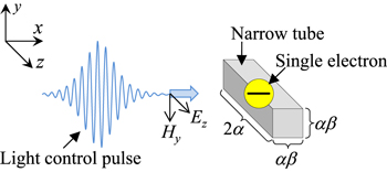
Figure 1. The geometry and coordinates of the studied system. A single electron is confined in a rectangular narrow tube placed parallel to the z-axis, with a degree of freedom only along this axis. The electronic properties of the narrow tube depend on the geometric parameters α and β. An incident light control pulse is a plane wave and is polarized along the z-axis.
Download figure:
Standard image High-resolution imageThe size and shape of this nanotube can be characterized by two parameters α and β; the α parameter specifies the length of the tube and has a unit of length in nanometers, while the dimensionless β parameter specifies the relative ratio between the length of the tube and the one-side length of its cross-section. For this system the time-dependent Schrödinger equation and the polarization current density ((1) and (4)) can be rewritten with mass m and charge q (= −e) of the electron as
where  denotes the unit vector along the z-axis. The wave function ψ in this Schrödinger equation is assumed to have finite probability density only within this tube. The incident light control pulse initially has only Ez and Hy components, before passing through the interaction region where the wave function spreads. All the other components of the electromagnetic field, however, need to be calculated, since immediately after the electron excitation the polarization current density creates the near-field, which has all the field components.
By changing the α and β parameters we can adjust the shape, size, and thus the electron density of the confined electron system thanks to the normalization condition, denoted as
The electrostatic confining potential V has been chosen to be a fourth power of z of the form

where V0 is set as 50 eV. The potential energy curve of V is plotted by the solid green line as displayed in figure 2, with the solid blue and broken pink lines denoting the probability density distributions of the ground and first-excited states, ψ0 and ψ1, that have been chosen in the present simulation to be the initial and objective states, respectively. This kind of single-well potential can mimic the confining potential of nanoscale objects such as quantum dots. In all cases the potential energy curve and thus the probability density distributions of the eigenstates have been kept similar to each other for different values of α. This similarity allows us to study the near-field effects for different α on an equal footing. The energy difference between the ground and the first-excited states for α = 0.5 is 21 eV. This rather large energy gap corresponding to an EUV photon energy has been chosen rather arbitrarily, but so as to save computational time. Although a more realistic choice may be a few electron-volts, corresponding to a visible light, the observed trends of the near-field effects in the present study depend little on the choice of energy gap.
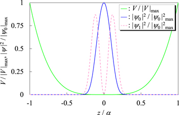
Figure 2. Spatial profile of the studied electrostatic potential V and the probability density distributions of the ground ψ0 state and of the first-excited ψ1 state. The potential V is shown in green and the probability density distributions for the ground and the first-excited states are displayed as solid blue and broken pink lines, respectively. The horizontal and vertical axes are normalized, respectively, by α and by its maximum value of V for the potential and of ∣ψ0∣2 for the probability density.
Download figure:
Standard image High-resolution imageThe computational scheme we employed here to perform the hybrid simulation of the coupled Maxwell–Schrödinger equations is based on the so-called finite-difference time-domain (FDTD) method [41–52] in which the electromagnetic field and the wave function are represented on discretized space and time grids. The operations of the space- and time-derivatives on these discretized field and wave functions are performed relying on their finite-difference formulas. The spacing for the x, y, and z coordinates, namely, Δx, Δy, and Δz, are related to α in the present study, so as to maintain the similarity of the potential energy curve among cases with different values of α as


The smaller value of Δz in comparison to Δx and Δy defined above has been chosen to assure high accuracy in the calculation of the wave function, since in the present quasi-one-dimensional model the wave function extends only along the z-axis as displayed in figure 1. In the FDTD scheme these spatial grid sizes restrict us to choose the time spacing Δt in order to perform stable and reliable propagation. We have employed the following Δt value, which is smaller by a factor of 0.9 than the value allowed by the so-called Courant–Friedrichs–Lewy condition [41, 52]:

One may refer to our previous study [41] where practical formulas to be used for coding the FDTD scheme in the hybrid simulation of the coupled Maxwell–Schrödinger equations were presented in detail in the appendix.
3. Results and discussion
As has been described in the previous section, we consider the physical situation where the ground state ψ0 is transferred to the first-excited state ψ1 by a light control pulse. Assuming that there is no polarization in the initial ground state, namely that there is a positive charge background compensating exactly the negative charge distribution of the electron at every spatial point as represented in equation (9), the NFR of equation (12) for the present system is rewritten as
where za is an arbitrary point in the tube along the z-axis while  represents the electric field of the light control pulse designed using the conventional scheme [35]. The conventional pulse is obtained by solving the following simultaneous equations:


where E0 and  represent, respectively, the amplitude parameter of the laser pulse and the wave function in the length gauge [53]. This procedure to obtain the light control pulse is derived through a more general formulation based on the optimal control theory and one can find detailed explorations of the topic in previous studies [32–35].
The conventional light control pulse designed using the above procedure shows us the influence of the near-field through its resultant control performance obtained in the hybrid Maxwell–Schrödinger simulation, since it has been designed neglecting the disturbance of the control pulse by the near-field. In the following subsections we explore the various physical situations and establish the relation between the values of the NFR and the influence of the near-field.
3.1. Dependence on electron density
In this subsection we investigate the influence of the near-field on the control of quantum states and establish a relation between the results and the corresponding values of the NFR by changing the β parameter from 0.5 to 1.5 while α is fixed as 0.5 nm. With this β variation we can change the probability density of the electron wave packet and thus study the effect of electron density on near-field generation. The amplitude parameter E0 in this subsection is fixed as 4.75 GV m−1. As will be demonstrated in sections 3.2 and 3.3, the choice of E0 is reflected in the pulse width. For large (small) values of E0 the control pulse is short (long). Therefore, fast control can be achieved in general by a strong laser pulse. On the other hand, in real systems such strong laser pulses may damage the target system. In this study we have chosen this value of E0 = 4.75 GV m−1 rather arbitrarily such that the laser pulse is not too strong yet capable of finishing the control within a dozen cycles of oscillation of the electric field of the laser pulse.
The temporal profiles of the light control pulses designed for the two typical cases with β = 0.5 and 1.5 are displayed in figure 3. This figure shows that these two pulses overlap each other completely, indicating that the conventional light control pulse does not account for the difference in the electron density of the target system. This happens because the conventional pulse designing scheme does not take into account the local modification of the laser pulse by the near-field. We note, however, that a larger electron density in matter in general gives a larger near-field, which could disturb the incident laser pulse more significantly.
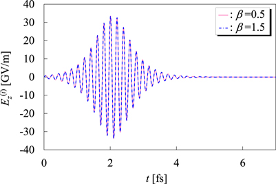
Figure 3. Temporal profile of the light control pulses  designed by the conventional method with no near-field effect taken into account. This pulse is designed to completely transfer the probability density of the electron from the ground state to the first-excited state for an electron confined in the electrostatic potential V (see figure 2). The solid pink and broken blue line represent the temporal profiles of the pulses designed for the conditions with β = 0.5 and 1.5, respectively. The other parameters α and γ are fixed, respectively, as 0.5 nm and 1.0.
Download figure:
Standard image High-resolution imageThe spatio-temporal propagation of the z-component of the electric field Ez (GV m–1) in the narrow tube computed by the Maxwell–Schrödinger hybrid simulation is displayed in figure 4 for the two cases with β = 0.5 and 1.5 that correspond to the results of the light control pulses shown in figure 3. In the case of figure 4(a), corresponding to the case with β = 0.5, there appears to be a significant disturbance of the incoming plane-wave form of the electric field around the center of the tube within ∣z/α∣ < 0.25, where the electron wave packet and thus the polarization current density have appreciable amplitudes. This result indicates that the confined electron feels an electromagnetic field which is largely different from the original laser pulse, and that the light control pulse designed by the conventional scheme therefore shows a significantly low controllability. In the case of the result in figure 4(b), corresponding to the case with β = 1.5, on the other hand, there seems to be only a small modification of the incoming the electric field, which is distorted weakly at around ∣z/α∣ < 0.25. The origin of these two distinct results can be rationalized as the difference in the electron density, as has been observed in our previous study [41]: according to the normalization condition of equation (15) the amplitude of the wave packet is inversely proportional to the β parameter. Then, the amplitude of the wave packet is directly reflected in the amplitude of the polarization current density by equation (14). Therefore, the influence of the local modification to the incident laser pulse is strongly dependent on β.

Figure 4. The spatio-temporal propagation of the z-component of the electric field Ez (in GV m–1) on the space grid located in the nanotube. In both the upper and lower panels the vertical axis represents Ez, while those extending right-to-left and front-to-back represent, respectively, the α-normalized z-coordinate (see figure 1) and time t (in fs). (a) and (b) show the results obtained using the Maxwell–Schrödinger hybrid simulation for the pulses designed under the conditions with β = 0.5 and 1.5, respectively. Blue and red represent high intensity in the electric field.
Download figure:
Standard image High-resolution imageA more detailed investigation of the dependence of the near-fields on β was undertaken and the result is summarized in figure 5. In this figure we have plotted NFR and the time-averaged square-modulus of the overlap between the objective state ψ1 and the electron wave packet after the pulse has gone (denoted by  for different values of β. The reason why we have taken a 'time-average' of this square-modulus of the overlap is due to the behavior of the electron wave packet in the Maxwell–Schrödinger hybrid scheme, whose components continue to oscillate if the control is incomplete. We note that this behavior is different from the oscillation of the time-dependent wave packet in the conventional framework of employing only the time-dependent Schrödinger equation. In the latter case the magnitude of each component remains unchanged after the pulse has gone and only their relative phases change in time, which results in the oscillation of the wave packet. In the present case, on the other hand, thanks to the coupling between Maxwell's and Schrödinger equations the oscillatory electron wave packet creates a near-field that modulates the relative strength in their components by repeated excitation and de-excitation as observed in our previous study [41]. A clear relation between
  and the NFR can be established by the results in figure 5: as β increases,
  which directly indicates the control accuracy with 1.0 for the highest and 0.0 for the lowest accuracies, is improved while the NFR decreases. More precisely, when the NFR is low, such as below 0.5,
  is over 0.9, indicating a high control accuracy. On the other hand, when the NFR is high, such as over 1.5,
  is in the range between 0.1 and 0.2, indicating that the control accuracy is quite low. This simple correspondence between the NFR and the control accuracy suggests that we can predict the near-field influence by simply calculating the NFR from equation (20). In the following subsections we consider other situations and show that this relation between the NFR and
  applies commonly.
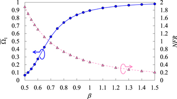
Figure 5. Correspondence between the NFR and the controllability for different values of the geometry parameter β controlling the electron density. The controllability  has been evaluated by the time-averaged square-modulus of the overlap between the electron wave packet and the objective first-excited state after the control pulse has gone and is indicated by blue circles. The NFR is indicated by pink triangles. The left- and right-hand sides of the vertical axes represent the scales for
  and NFR, respectively.
Download figure:
Standard image High-resolution image3.2. Dependence on the amplitude of the control pulse
In the previous subsection the dependence of the near-field on the β parameter, which controls the electron density of the target system, has been investigated. In this subsection the relation between the NFR and the control accuracy is demonstrated, focusing on its dependence on the characteristics of the laser pulse; more precisely, the dependence on the amplitude and thus the pulse width of the light control pulse. This can be achieved by introducing a dimensionless scaling parameter γ to the amplitude parameter of the laser pulse E0 in equation (21) as

where  represents the amplitude parameter for the 'normal' case with (α, β) = (0.5, 1.0) and has the value of 4.75 GV m−1 as noted in the previous subsection. The geometry parameters α and β are kept constant throughout this subsection.
As was done in the previous subsection, we first demonstrate the results for two typical cases obtained by the Maxwell–Schrödinger hybrid simulation. Figure 6 shows the temporal profile of the light control pulses designed for γ = 0.2 and 2.0. In the case of γ = 0.2 the pulse width becomes longer than that displayed in figure 3 while in the case with γ = 2.0 it becomes shorter. This difference is due to the fact that any pulses designed to transfer the electronic state from its ground state into the first-excited state completely, have to contain the same amount of electromagnetic energy. Thus, the light control pulse for γ = 0.2 having a small amplitude has to be broad while that for γ = 2.0 having a large amplitude is short.
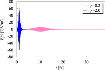
Figure 6. Temporal profiles of the light control pulses  for different values of the scaling parameter γ (see equation (23)). The pink solid and blue lines represent, respectively, the light control pulse for γ = 0.2 and 2.0. The geometry parameters of the confined electron systems, α and β, are fixed as 0.5 nm and 1.0, respectively.
Download figure:
Standard image High-resolution imageAs was done in figure 4, we have calculated the spatio-temporal propagation of Ez in the narrow tube for these two light control pulses and the results are displayed in figures 7(a) and (b) for γ = 0.2 and 2.0, respectively. The result for γ = 0.2 (figure 7(a)) shows that the incident plane-wave electric field is disturbed so strongly around the region ∣z/α∣ < 0.25 that even a clear node appears in this region as a result of interference between the original laser field and the near-field. In contrast, the result displayed in figure 7(b) for γ = 2.0 shows only a weak modification of the incident electric field, which becomes recognizable only after the pulse has started to decay after t > 1.0 fs. These observations can be rationalized as follows. As we noted in section 2.2, the near-field becomes largest when perfect control is achieved, namely, when the dynamic polarization in the charge-density distribution of the target electron system is largest. Therefore, in optical-control problems the upper bound of the near-field strength is governed purely by the electronic property of the matter and is independent of the characteristics of the laser pulses. The increase in the amplitude of the laser pulse, therefore, leads to a relative decrease in the amplitude of the near-field with respect to the incident laser field and thus a decrease in the near-field effect, as observed in figure 7(b).
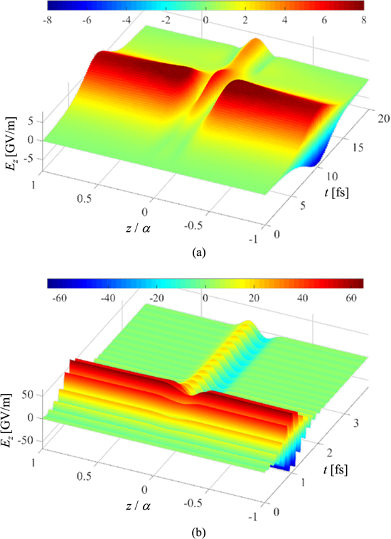
Figure 7. The spatio-temporal propagation of the z-component of the electric field Ez (in GV m–1) obtained by the Maxwell–Schrödinger hybrid simulation for different values of the γ parameter controlling the amplitude of the light control pulses. (a) and (b) show the results for the light control pulses designed under the conditions with γ = 0.2 and 2.0, respectively. See the caption to figure 4 for further details.
Download figure:
Standard image High-resolution imageAs has been done in figure 5, the correspondence between the NFR and the control accuracy  measured by the time-averaged square-modulus of the overlap between the electron wave packet and the objective state after the pulse has gone, is displayed in figure 8 for different values of γ ranging from 0.2 to 2.0. The results displayed in this figure support our reasoning: the control accuracy is improved for increasing γ and decreasing NFR and vice versa. The practically useful relationship between the NFR and the controllability of the light control pulse, which was explored in the previous subsection, can also be verified in the result of figure 8: when the value of the NFR is less than 0.5, the controllability of the light control pulse can be high with the
  value >0.9. On the other hand, when the NFR value is over 1.5, the controllability becomes quite low with
  as small as <0.1.
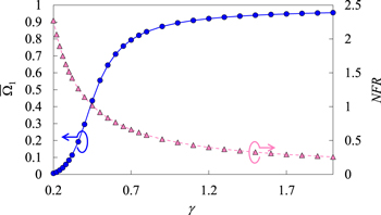
Figure 8. Correspondence between the NFR (indicated by circles) and the controllability (triangles) of the light control pulse for different values of the γ parameter determining the amplitude of the incident pulse (see equations (21) and (23)). See the caption to figure 5 for further details.
Download figure:
Standard image High-resolution image3.3. Dependence on the length of the tube
In this subsection we investigate the influence of the near-field with respect to variation of the α parameter, which appears in equations (15)–(18), while keeping both β and γ as 1.0. By doing so we can examine its dependence on the length of the tube as displayed in figure 1. In the previous two subsections the dependence of the near-field effect on the electron density and on the characteristics of the light control pulse was studied by changing β and γ independently. However, when the α parameter is varied, as in this section, not only the electron density but also the energy gap between the ground and first-excited states, δE, changes since the confinement strength has been changed. A change in the energy gap between the target quantum states would naturally lead to a change in the frequency components involved in the light control pulse. Furthermore, we note that the integration range za to evaluate equation (20) would also be changed for different α since the extent of the electron wave packet become larger for larger α. This would result in another effect, since the electron wave packet oscillating in a wider spatial range would give a larger polarization and thus a larger near-field effect. Therefore, we can examine the interplay among the three different effects associated with the change in the electron density, the characteristics of the laser pulse, and the extent of the electron wave packet.
We note that the changes in the electron density, the control pulse, and the length of the electron wave packet along the polarization axis for different α contribute to the NFR in different ways. As α increases the confinement for the electron becomes weaker. At the same time, the cross-section of the tube becomes larger, as shown in figure 1. Therefore, the NFR would tend to decease for increasing α when considering only the change in the electron density. However, as α increases, the energy difference δE between the ground and the first-excited states becomes smaller owing to a weaker confinement, which results in the lowering of the resonance frequency. Then, the amplitude of the light control pulse decreases as its pulse width becomes longer. As has been demonstrated in section 3.2, such a decrease in the amplitude of the incident pulse leads to an increase in the NFR. Third, the increase in α leads to a longer electron wave packet along the z-axis and thus a larger polarization. This results in an increase in the value of the NFR.
The temporal profiles of the light control pulses designed for α = 0.5 and 1.5 are displayed in figure 9(a). The pink solid line corresponding to α = 0.5 in this figure shows a significantly larger amplitude and a higher central frequency than the blue line representing the case with α = 1.5. This difference is a consequence of the change in the strength of confinement, as has been explained above. Both pulses, however, can agree with each other when they are normalized such that the time t and the electric field  are divided by the cycle T
  and its maximum amplitude, respectively, as shown in figure 9(b). In order to maintain the shapes of the pulses as identical after this normalization we have employed the following form of the amplitude parameter that involves δE as

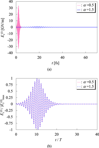
Figure 9. Temporal profiles of the light control pulses  designed under the conditions with different values of the α parameter determining the length of the tube (see equations (16)–(18)). The pink solid and blue lines correspond, respectively, to the cases with α = 0.5 and 1.5. The pulses displayed in (a) are represented in a normal scale, while those in (b) are normalized such that the horizontal and vertical axes are scaled, respectively, by the cycle T of oscillations and by the maximum field amplitude. The other parameters characterizing the system β and γ are both fixed as 1.0.
Download figure:
Standard image High-resolution imageThis agreement allows us to make a fair comparison among the cases with different α, focusing on the interplay between the effects of the electron density, the amplitude of the laser pulse or its pulse width, and the extent of the electron wave packet.
The spatio-temporal propagation of the resultant Ez obtained by the Maxwell–Schrödinger hybrid simulation for the cases with α = 0.5 and 1.5 is displayed in figures 10(a) and (b), respectively. In both figures the time and the field amplitude are normalized as in figure 9(b). The results displayed in figure 10(a) for the case with α = 0.5 show that the electric field of the incident laser pulse is modified weakly by the near-field after t/T ≥ 10, suggesting that the controllability of the pulse would be decreased only a little by this modification. On the other hand, the result in figure 10(b) corresponding to the case with α = 1.5, shows that the incident electric field is modified significantly around the electronic wave function, namely in the vicinity of the region ∣z/α∣ < 0.25, and that the amplitude of the electric field at around t/T ∼ 10 becomes very weak owing to destructive interference with the near-field. This result suggests that a larger α value would result in lower controllability, or in other words, a larger value of the NFR.

Figure 10. The spatio-temporal propagation of the z-component of the normalized electric field Ez obtained by the Maxwell–Schrödinger hybrid simulation for different values of the α parameter determining the length of the nanotube. (a) and (b) show the results for the conventional light control pulses designed under conditions with α = 0.5 and 1.5, respectively. In both figures the vertical axis is normalized by the maximum field amplitude, while those extending right-to-left and front-to-back are scaled, respectively, by the cycle T of oscillations and the α parameter. See the caption to figure 4 for further details.
Download figure:
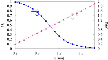
Standard image High-resolution imageWe have performed similar simulations and calculated the NFR by changing the α value gradually in the range between 0.2 and 2.0. The controllability of the light control pulses has also been evaluated by calculating the time-averaged square-modulus of the projection of the final electron wave packet on the objective state  , as was done in figures 5 and 8. The result is displayed together with the value of the NFR in figure 11. As α increases, the controllability of the laser pulse
  decreases, while the NFR increases linearly. This result indicates that the dependence of the near-field effect on the characteristics of the light pulse, particularly its amplitude, or on the extent for the electron wave packet, is more dominant than that of the electron density in the present model system. As was done in the previous two subsections, we have examined the relationship between the values of the NFR and
  The result shows the same tendency as in the previous two cases: good controllability of the light control pulse
  can be assured for NFR ≤ 0.5, while it becomes significantly low
  for NFR ≥ 1.5. This result, together with those of the previous two subsections, suggests that the NFR can be an indicator to preliminarily estimate the influence of the near-field. This would enable us to judge whether to stay with the standard time-dependent Schrödinger equation (with low computational cost), or use the precise but complicated Maxwell–Schrödinger hybrid method, when using numerical simulations to design light control pulses for the optical control of quantum systems.
Figure 11. Correspondence between the NFR (indicated by circles) and the controllability (triangles) of the light control pulse for different values of the α parameter determining the length of the nanotube (see figure 1 and equation (16)). See the caption to figure 5 for further details.
Download figure:
Standard image High-resolution image
Finally, we have summarized the ranges of parameters characterizing the light control pulses exploited in the present study. The field intensity of the light control pulses ranged from ∼1010 W cm−2 (weak field) to ∼1015 W cm−2 (strong field). The one-photon energy varied in the range between 1 to dozens of electron-volts depending on the strength of confinement for the target electron systems. These parameter ranges cover the photon energy and intensity ranges of interest in the current experiments using ultrashort laser pulses. Therefore, the present demonstration of the NFR can be of practical use in the estimation of the magnitude of the near-field effect in optical control of confined electron systems.
4. Summary
In this paper we have proposed a simple formula that can estimate the magnitude of disturbance of the incident laser pulse by the near-field in optically controlled confined electron systems. This formula can be easily used without involving elaborate computation and thus allows us to judge whether to solve the time-consuming coupled Maxwell–Schrödinger equations or to stay with the standard time-dependent Schrödinger equation approach that accounts for no such near-field effect.
We started our discussion with consideration of the most significant situation where complete optical control, namely complete transfer of the probability density from one state to another by a light control pulse, is achieved. Such a complete transfer of the probability density gives rise to a charge-density polarization between the initial and the final states. The maximum strength of the electric field owing to this charge-density polarization can be a measure of the upper bound of the magnitude of the near-field created in the vicinity of the excited electron. We then introduced the concept of the near-field ratio (NFR), a simple formula, as a measure to judge the significance of the disturbance of the light control pulse by the near-field. The NFR is defined as the ratio of the maximum strength of the electric field due to the charge-density polarization over that of the incident light control pulse.
In order to demonstrate the applicability of the NFR we have focused on a system of an electron confined in a quasi-one-dimensional nanoscale potential well. The light control pulse, which aims to transfer the probability density of the electron completely from its ground state to the first-excited state, was designed using the conventional scheme, which takes no near-field effect into account. The controllability of this light control pulse was examined by performing the Maxwell–Schrödinger hybrid simulation and evaluating the probability of reaching the objective of the first-excited state for different values of the parameters characterizing the studied system. We have identified the ranges of the value of the NFR where the controllability of the conventional light control pulse is high and where it is significantly low. When the NFR is lower than 0.5, the probability of reaching the target state can be larger than 0.9, indicating that we may use the conventional light control pulse that neglects the near-field effect. On the other hand, when the NFR is larger than 1.5, the probability of reaching the target state can be as low as <0.1, indicating that the conventional scheme for designing light control pulses does not work, and that we have to employ the Maxwell–Schrödinger hybrid scheme in designing control pulses, as we proposed in our previous study [41]. We have thus obtained an indicator for use of the Maxwell–Schrödinger hybrid simulation in optical-control problems.
Acknowledgments
The authors would like to thank Professors K Nakagawa, Y Ashizawa (Nihon University), and M Tanaka (Gifu University) for their useful comments and suggestions. This work was partly supported by Grant-in-Aid for Scientific Research (C) (No. 26420321) and MEXT-Supported Program for the Strategic Research Foundation at Private Universities, 2013–2017. One of the authors (T S) also acknowledges MEXT for financial support (Grants-in-Aid for Scientific Research (C) (No. 15K05396) and Grants-in-Aid for Scientific Research on Innovative Areas (No. 25110006)).
Appendix
In this appendix we present the mathematical formulas to be used in finding the initial conditions for the electric field E and scalar potential φ in the situation where the electron system is initially polarized, as mentioned in section 2.2, namely,

The following equations have to be satisfied when the system initially includes the polarization charge density at t = 0:


where Es and φs then are the initial values for the electric field and scalar potential, respectively.
We can rewrite equations (A1) and (A2) into a single formula as

By determining the polarized initial condition  namely setting C involved in equation (8), this Poisson's equation is solved by a standard computational technique, such as constructing a representation matrix for the Laplacian operator on the spatial grid and applying its inverse matrix to the right-hand side of equation (A3) (for more details see the appendix in [37]). The electric field is then obtained by taking a gradient of the resultant scalar potential, as in equation (A2).