
Abstract
The spin reorientation temperature TSR of stoichiometric Fe3O4, as well as of magnetite with a small number of vacancies and magnetite containing a low concentration of Ti, Zn, Al and Ga was measured on single-crystal samples using the ac susceptibility. In the same experiment the temperature TV of the Verwey transition was also found. The results show that a correlation between TSR and TV exists. The electronic structure of the compounds studied was determined using the density-functional-based GGA + U method. For stoichiometric magnetite the first and second cubic anisotropy constants were calculated, while for magnetite with defects the distribution of electron density using the 'atoms in molecules' approach was determined. Based on a combination of experimental results with the electronic structure calculations an explanation of the temperature dependence of the magnetocrystalline anisotropy of magnetite is suggested.
Export citation and abstract BibTeX RIS
1. Introduction
Temperature dependence of the magnetocrystalline anisotropy of magnetite was the subject of numerous studies in the past (for a survey see [1]). In the cubic phase, above the Verwey transition, the anisotropic part Ean of the energy is well described by the first and second anisotropy constant K1 and K2:

where ϑx,ϑy,ϑz are direction cosines of the magnetization. Unlike the magnetization, the magnitude of which increases monotonically with decreasing temperature, the K1(T) and K2(T) dependences are nonmonotonic. K1 is negative at ambient temperature; it first decreases with decreasing temperature, acquiring a minimum at T ≃ 250 K. It then increases and becomes positive at the spin reorientation temperature TSR, which is slightly higher than the temperature TV of the Verwey transition. The temperature dependence of K2 is similar [2]. Abe et al [3] suggested to decompose K1(T) into a monotonically decreasing, negative, term  and a positive, anomalous, part ΔK1:

Below TV the crystal symmetry is monoclinic with the space group Cc and the anisotropy is described by

where ϑa and ϑb are the direction cosines with respect to the monoclinic a and b axes, and  with respect to the axis
 ![$[\bar {1}01]$](https://content.cld.iop.org/journals/0953-8984/24/5/055501/revision1/cm407531ieqn29.gif) of the monoclinic system defined in [3] (i.e. the elongated body diagonal of cubic cell). The values of the anisotropy constants at 4.2 K, determined experimentally by Abe et al [3], are (in 104 J m−3)
of the monoclinic system defined in [3] (i.e. the elongated body diagonal of cubic cell). The values of the anisotropy constants at 4.2 K, determined experimentally by Abe et al [3], are (in 104 J m−3)

and below TV the anisotropy energy is thus dominated by the second-order term proportional to Ka. The fourth-order terms in  may be averaged [3] to obtain an analog of the cubic K1 constant:

The  temperature dependence smoothly connects to
  extrapolated from the cubic phase. The situation is shown in figure 1 adapted from [1].
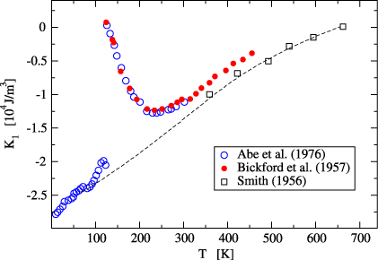
Figure 1. Temperature dependence of the magnetic anisotropy constant K1 in magnetite. The dashed line is an estimation of the K1(T) dependence using the high temperature data of Smith [7] and low temperature  data of Abe et al [3]. Adapted from [1].
Download figure:
Standard imageThere were several attempts to explain the increase of K1 below 250 K. Abe et al [3] connected ΔK1 with the possible presence of strongly anisotropic ions, the most probable candidate being Fe2+. Siratori and Kino [4] proposed that ΔK1 originates from a short range ordering of Fe2+ ions on the octahedral sublattice that presumably appears above TV and becomes stronger as temperature decreases. As pointed out by Ka̧kol and Honig [2] both these suggestions are rather improbable. These authors showed that the deviation from ideal stoichiometry influences the anisotropy only slightly, despite the fact that the resulting increase of the mean valency of Fe(B) ions reduces the number of (hypothetical) ferrous ions on the octahedral sites. Also the nuclear magnetic resonance (NMR) results [6] showed that, if any short order exists, it must be dynamic, with a characteristic frequency larger than ∼100 MHz.
Using thermodynamic considerations and the mean-field model Aragón [5] analyzed the temperature dependence of K1 in stoichiometric and slightly non-stoichiometric magnetite. He concluded that the anomalous term ΔK1(T) is caused by a degeneracy of the excited states, which should be twice the degeneracy of the ground state. The nature of the excited states was not specified by Aragón, however.
To achieve a deeper insight into the anisotropy of magnetite and magnetite containing defects we determined the spin reorientation temperature TSR using the ac susceptibility. TSR is very sensitive to the details of the temperature dependence of the anisotropy, yet its determination using ac susceptibility is relatively easy. In the same experiment the Verwey temperature is also determined. The systems studied comprise stoichiometric Fe3O4, magnetite with a small number of vacancies Fe3(1−δ)O4 and magnetite Fe3−xMxO4 containing a low concentration of M = Ti, Zn, Al and Ga. These substitutions, as well as the vacancies, represent 'charged' defects, i.e. they change the nominal valency of iron ions on the octahedral sites. In stoichiometric magnetite all tetrahedral (A) sites are occupied by ferric ions, while the formal valency of iron on the octahedral (B) sublattice vB is 2.5, so that formally its formula may be written as Fe3+(A)[Fe3+(B)Fe2+(B)]O4. Cation vacancies occur in the B sublattice [2] and to maintain charge neutrality more electron holes should appear on the B sublattice, i.e. according to the above formula part of Fe2+ becomes Fe3+. The stable valency of zinc is 2+ and it replaces trivalent iron on the A sites [9]. The presence of Zn thus again leads to an increase of Fe(B) valency. Another charged impurity is titanium, which is tetravalent and enters into the B sublattice [8]. In this case charge neutrality requires a decrease in the average valency of Fe(B) ions. Weaker influence on the charge distribution is from aluminum, which is trivalent and enters the B sublattice, providing its concentration is low [11]. The situation in magnetite containing Ga is more complex: Ga is trivalent and it preferentially occupies the A sites, though part may be found also in the B sublattice [12, 13]—the Fe(B) valency is therefore affected mostly by the Ga ions in the B sites.
We also calculate the anisotropy of stoichiometric cubic magnetite using the method based on the density functional theory. As such a calculation probes the energy of the system at absolute zero temperature, the calculated K1 corresponds to  of (5). Analogous determination of anisotropy in the defect-containing systems would be too demanding on the computing power. For these systems we calculate the electron and spin density distribution, which quantities are of considerable interest, especially when the defect is charged. In the gas of quasifree electrons the screening of a static point charge results in the Friedel oscillations. In the magnetite the situation is more complex. First, the extra charge is screened both by a local distortion of the crystal and by a redistribution of the electron density. Second, due to the half-metallic character of the compound, only the minority spin electrons are effective in screening the extra charge. Finally the 3d electrons of iron are correlated. An interesting question is whether the extra charge carriers induced by the charged defect remain localized on a single B sites close to the defect, or to which extent they become delocalized.
2. Experimental details
Chemical formulae of samples with cation substitution and non-stoichiometric samples are Fe3−xMxO4 and Fe3(1−δ)O4, where the x parameter stands for the concentration of substitution metal M and the δ parameter denotes the concentration of vacancies. Single-crystal samples were either prepared by the floating zone technique [8] or grown from the melt by using the cold crucible method [9]. The electron microprobe assisted in a determination of the concentration of the substitution. A list of studied samples is provided in table 1, where TV and TSR are also given.
Table 1. List of investigated compounds. Compounds denoted by an asterisk (*) were prepared by the floating zone method [8]; all other samples were grown from the melt by the cold crucible technique [9]. vB is a formal mean valency of Fe on the B sublattice. Spin reorientation TSR and temperature of the Verwey transition TV are in K. Although trivalent Ga ions preferentially occupy the A sites, part of them (xB ∼ 0.01 [13]) entering into the B sublattice was taken into account when calculating vB.
| Compound notation | x or δ | vB | TSR | TV |
|---|---|---|---|---|
| Pure* | 0.000 | 2.500 | 132.7 | 122.2 |
| Ga* | 0.050 | 2.497 | 126.7 | 117.5 |
| Zn1 | 0.007 | 2.504 | 124.0 | 113.2 |
| Zn2 | 0.009 | 2.505 | 122.5 | 110.0 |
| Zn3 | 0.017 | 2.509 | 121.0 | 104.3 |
| vac1 | 0.002 | 2.503 | 128.0 | 114.1 |
| vac2 | 0.009 | 2.511 | 124.0 | 101.0 |

|
0.008 | 2.494 | 128.0 | 116.4 |
| Ti2 | 0.008 | 2.494 | 126.0 | 119.0 |
| Ti3 | 0.020 | 2.485 | 110.0 | 79.1 |

|
0.005 | 2.499 | 128.3 | 119.7 |

|
0.030 | 2.492 | 126.5 | 97.3 |
As a suitable tool to determine TV and TSR we used the ac susceptibility at a zero applied static magnetic field (initial susceptibility). It was measured by a SQUID magnetometer MPMS-5S (Quantum Design) in ac magnetic field he = 0.3 Oe at frequency 1 Hz. Samples of approximately cylindrical form were used with the external driving ac magnetic field he directed along the longitudinal axis. The evaluated external complex susceptibility χe = χ'e − iχe'' = m/he was not corrected for demagnetizing effects depending on the sample dimensions. χe sensitively reflects the magnetic and electronic structure of the system, though the details of the underlying mechanism may be complex. In the past, temperature dependence of the susceptibility of stoichiometric Fe3O4 was studied by several authors. In particular Skumryev et al [10] showed that there is a clear anomaly in the χ'e(T) and χe''(T) at TV, while the spin reorientation transition manifests itself in a less pronounced maximum in χ'e(T) accompanied by a minimum in χe''(T). These authors also discussed the possible origin of the observed χe(T) dependence.
We studied the temperature dependence of χe in the temperature region of the Verwey transition, i.e. between about 70 and 140 K, and found that in all samples its behavior is similar to the one of stoichiometric magnetite. A typical example is displayed in figure 2. The temperature of the Verwey transition TV was determined as a point of maximum first derivative dχ'e/dT. This temperature corresponds approximately to a maximum of the imaginary part χe''. For low concentration of defects the increase of the susceptibility is abrupt which suggests the first-order character of the transition. Above a critical concentration the character of the χ'e(T) becomes continuous, pointing to the second-order character of the phase transition [2]. Above the Verwey transition the real part of the susceptibility increases with increasing temperature and at T = TSR it passes through a maximum (at this temperature we also observed a less pronounced minimum of the χe''(T)). This temperature was taken as a spin reorientation temperature.
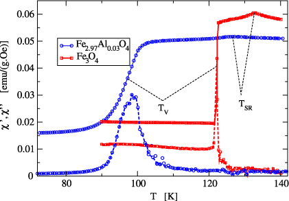
Figure 2. Temperature dependence of the real (full curves) and imaginary (dashed curves) parts of the external susceptibility for the pure magnetite and Fe2.97Al0.03O4 (sample Al2 in table 1). The imaginary part was multiplied by a factor of 50.
Download figure:
Standard imageOur measurements were performed during warming the samples after verifying that for pure magnetite the temperature hysteresis between TV measured during warming and cooling seems to be finite but less than 0.1 K. This is in accord with the hysteresis 0.03 K obtained from the measurements of the specific heat [14]. In our experiments no hysteresis was found at the temperature TSR.
The dependence of TSR and TV on the mean valency of Fe(B) ions is displayed in figure 3. We also studied in all 12 systems the temperature dependence of the 57Fe NMR spectra. The results will be published elsewhere; here we only mention that TV determined by NMR agrees well with the value obtained from the ac susceptibility.
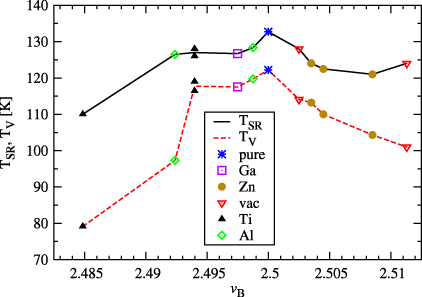
Figure 3. Dependence of spin reorientation temperature TSR and temperature TV of Verwey transition on the average valency vB of iron ions on the octahedral sites. The lines serve only as guides for the eyes.
Download figure:
Standard image3. Calculations
The electronic structure of the respective compounds was calculated using the augmented plane wave + local orbital method based on the density functional theory as implemented in the WIEN2k program [15]. For the exchange–correlation functional the generalized-gradient approximation form [16] was adopted. To improve the description of iron 3d electron correlations we used the rotationally invariant version of the LDA + U method as described by Liechtenstein et al [17], with the GGA instead of LSDA exchange–correlation potential and with a single parameter Ueff = U − J only. In most of the calculations described in what follows, Ueff = 4.5 eV, which value was successfully used to explain the contact hyperfine field in a number of iron oxides [18]. The radii of the atomic spheres were chosen as 1.6 au for oxygen and 1.8 au for the cations. The number of basis functions was ∼100/atom (RKmax = 7.0), and the charge density was Fourier-expanded to  .
.
In all cases considered the band structure corresponds to a half-metal: the density of minority spin states is nonzero on the Fermi energy, while there is a gap in the density of the majority spin states. The magnitude of this gap increases with increasing Ueff and for Ueff = 4.5 eV it amounts to 2.28 eV in the stoichiometric magnetite. In the defect-containing Fe3O4 the value of the gap is reduced, being 2.02, 1.87, 1.76, 1.55 and 1.38 eV for Ga(A), vacancy(B), Zn(A), Al(B) and Ti(B), respectively. The magnitude of the gap is important for the eventual application of magnetite in spintronics.
3.1. Magnetocrystalline anisotropy
Calculation of the magnetocrystalline anisotropy of ferric compounds which possess cubic symmetry is a formidable problem—the anisotropy is small as a rule and calculated results are sensitive to the method used, as well as to the parameters of the calculation (number of the k-points, number of the basis functions, form of the exchange–correlation functional, etc). This concerns the first anisotropy constant K1 and it presents an even more serious problem for the second and higher anisotropy constants. K1 of the stoichiometric magnetite was calculated by Jeng and Huo [19], who used the local-spin-density approximation, as implemented in the linear muffin-tin orbital method [20]. No attempt was made to improve the description of the electron correlation by employing the LDA + U method.
In view of the differences between our and [19] theoretical methods we recalculated the anisotropy of the cubic magnetite using the force theorem (for a recent discussion of the force theorem and further references see [21]). The spin-polarized calculation is first converged; then the magnetization direction [hkl] is specified and the eigenvalue problem with a converged potential and the spin–orbit coupling switched on is solved. Finally the sum of eigenvalues Ehkl up to the Fermi energy is evaluated for different [hkl] and used to determine the anisotropy. In cubic systems three calculations with magnetization along [001], [111] and [110] symmetry directions are sufficient to determine the first and second anisotropy constant:

The key problem in calculating the magnetocrystalline anisotropy is its dependence on the number Nk of k-points in which the eigenvalue problem is solved. For Ueff = 4.5 eV this dependence is displayed in figure 4. To see the role of third- and higher-order anisotropy constants, the calculation was also performed for  [113] and the resulting E113 subtracted from the anisotropy energy
  calculated using K1,K2 of (6). The result

is also displayed in figure 4. As seen from this figure K1 is negative and reasonably converged for Nk ≳ 7000, which to a lesser extent holds also for K2. The energy difference D113 is small, indicating that the anisotropy is well approximated using only two anisotropy constants.
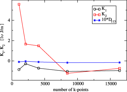
Figure 4. Calculated anisotropy constants of the stoichiometric Fe3O4 as functions of the number of k-points in the irreducible wedge of the Brillouin zone.
Download figure:
Standard imageThe dependence of K1 and K2 on the parameter Ueff is shown in figure 5. As the calculation with Nk = 16 400 (corresponding to the division of the Brillouin zone 40, 40, 40) represented the upper limit of our computer possibilities, this dependence was determined by adopting Nk = 8448 (division 32, 32, 32). The value of the first anisotropy constant extrapolated to Ueff → 0 is −2.1 × 10⁴ J m−3, which is surprisingly close to −2.7 × 10⁴ J m−3 obtained by Jeng and Guo [19].

Figure 5. Calculated anisotropy constants of the stoichiometric Fe3O4 as functions of the parameter Ueff.
Download figure:
Standard image3.2. Magnetite with defects
The experimentally studied compounds were modeled by supercells 2 × 2 × 2, where one iron atom was substituted by Zn, Ti, Al, Ga or removed. Denoting the defect as X, the formula is Fe47XO64, corresponding to the defect concentration 0.0625, which is not far from the situation in the studied samples. The unit cell contains 112 atoms (111 atoms for magnetite with the vacancy). Internal positions in all structures were optimized by minimizing the forces exerted on the atoms. The calculations were performed in 28 k-points in the irreducible part of the Brillouin zone. In all cases the value of the parameter Ueff = 4.5 eV was adopted.
Properties of interest is the distortion of crystal lattice around the defect as well as the change of charges and magnetic moments of neighboring atoms. In a standard FPLAPW calculation atomic charges and spin moments are evaluated in a simple way as a sum or difference of spin-up and spin-down electron density within the given atomic sphere. Then, however, the contribution of the density in the interstitial region is disregarded and the result depends to some extent on the atomic radii. More correctly, the atom can be considered as a generalized volume around the nucleus, in the sense of the atoms in molecules approach (AIM) [22], charge and magnetic moments are then evaluated within such a volume. The results are given in tables 2–4.
Table 2. Stoichiometric Fe3O4. Atomic valence charges q determined by the AIM method (in units of electron charge) and spin magnetic moments ms (in Bohr magnetons). q is calculated as the difference of the atom's atomic number and the charge contained in the AIM volume.
| Atom | |||||
|---|---|---|---|---|---|
| Fe(B) | Fe(A) | Oxygen | |||
| q | ms | q | ms | q | ms |
| 1.624 | 3.955 | 1.804 | 4.106 | −1.261 | 0.049 |
Table 3. Atomic valence charges and spin magnetic moments in defect-containing magnetite. X, Fe(B)nn, Fe(A)nn, Onn, Fe(B)nnn correspond to the defect, its nearest Fe(B) neighbor, Fe(A) neighbor, oxygen neighbor and the next-nearest Fe(B) neighbor. q and ms have the same meaning as in table 2, in which the data for the pure magnetite are given.
| X | Fe(B)nn | Fe(A)nn | Onn | Fe(B)nnn | ||||||
|---|---|---|---|---|---|---|---|---|---|---|
| Defect | q | ms | q | ms | q | ms | q | ms | q | ms |
| Ga3+(A) | 1.873 | 0.026 | 1.537 | 3.825 | 1.761 | 4.109 | −1.293 | 0.175 | 1.633 | 3.953 |
| Zn2+(A) | 1.275 | 0.052 | 1.644 | 3.984 | 1.755 | 4.091 | −1.277 | 0.266 | 1.791 | 4.153 |
| vac(B) | 1.712 | 4.033 | 1.772 | 4.097 | −1.188 | 0.008 | 1.701 | 4.041 | ||
| Ti4+(B) | 2.252 | 0.087 | 1.423 | 3.634 | 1.770 | 4.111 | −1.246 | −0.051 | 1.797 | 4.155 |
| Al3+(B) | 2.561 | 0.009 | 1.445 | 3.642 | 1.767 | 4.114 | −1.364 | −0.071 | 1.624 | 3.939 |
Table 4. Equilibrium distances in defect-containing (lines 2–5) and stoichiometric magnetite (lines 6–7) in nm.
| Fe(B)nn | Fe(A)nn | Onn | Onnn | |
|---|---|---|---|---|
| Ga3+(A) | 0.3454 | 0.3658 | 0.1848 | 0.3535 |
| Zn2+(A) | 0.3451 | 0.3647 | 0.1963 | 0.3534 |
| vac(B) | 0.2804 | 0.3506 | 0.2200 | 0.3564 |
| Ti4+(B) | 0.3025 | 0.3485 | 0.1976 | 0.3651 |
| Al3+(B) | 0.2947 | 0.3457 | 0.1939 | 0.3564 |
| Fe(B) | 0.2967 | 0.3480 | 0.2059 | 0.3565 |
| Fe3+(A) | 0.3480 | 0.3635 | 0.1887 | 0.3493 |
4. Discussion
The results of electronic structure calculations presented in section 3.2 are a convenient starting point for a discussion of the physics of defect-containing magnetite. The data in table 3 show that ferric ions on the tetrahedral sublattice are almost intact by the defect, the largest difference in their valence charge in the systems studied being ∼1%. As expected, the iron ions on the octahedral sites are much more affected, the difference in their valence charge, relative to the stoichiometric magnetite (see table 2), ranging from −12% to +5% for the defect's nearest Fe(B) neighbors. For the next-nearest Fe(B) neighbors of the defect this difference lies between −0.2% and +11%. Note that there is also an appreciable change of the charge of the nearest oxygen neighbors to the defect. Larger supercells will be necessary, however, in order to find whether an analog of the Friedel oscillations in magnetite exists.
Inspection of table 4 reveals that a considerable part of screening is due to the local distortion around the defect. Both Zn2+ and the vacancy on the B site carry negative charge relative to Fe(B) and thus the nearest oxygen ions are repelled. The distortion is particularly large around the vacancy, for which the distance to the nearest oxygen is increased by ∼7%. As expected the Ti4+ ion on the B site causes the contraction of the octahedron. A somewhat stronger contraction is associated with Al3+(B). In this case the attraction caused by the Coulomb interaction is upheld by the smaller ionic radius of Al3+ (0.0675 nm) compared with the ferrous and ferric ions (0.092 and 0.0785 nm [23]).
The above-described results show that in the ground state of the defect-containing cubic magnetite the modification of the charge density spreads over a considerable distance. As a consequence no localized, strongly anisotropic ions are present. It is thus understandable why the magnetocrystalline anisotropy and hence also the temperature of spin reorientation (table 1) is only weakly modified by the presence of defects. Figure 3 suggests strongly that the Verwey and spin reorientation transitions are correlated. The difference between TSR and TV is ∼10 K for stoichiometric magnetite or low concentration x of the defects (namely for small deviation of average valency vB of iron in octahedral sites from the stoichiometric value 2.5) and it increases up to ∼30 K when x (and thus also the difference vB − 2.5) is larger.
The calculated first anisotropy constant has the same sign, but its magnitude is ∼2 times smaller comparing to  (cf figures 1 and 5). As noted by Brabers [1] the magnitude of
  may be too large because the high temperature data of Smith [7] were used in the extrapolation. Part of the discrepancy could also be connected with an underestimation of the orbital moment, which is often encountered in the density-functional-based calculations. In view of these uncertainties the agreement between calculated K1 and
  is reasonable.
Attention can now be turned to the anomalous part ΔK1 of the cubic first anisotropy constant. The fact that both  obtained by the extrapolation of the experimental data and K1 calculated by GGA + U are negative, while ΔK1 is positive, shows that ΔK1 is connected to the degeneracy of the excited state present in the cubic phase only. This agrees with the hypothesis of Aragón [5] who, however, avoids specifying the nature of this state. Figure 3 indicates a strong correlation between the spin reorientation transition (and thus anisotropy) and the Verwey transition. This leads us to suggest that the excited state corresponds to a local charge and orbital ordering that becomes long range and stable for T < TV. It will be degenerate as several orderings are equivalent in the cubic symmetry. Assuming that there is a one-to-one correspondence between the Cc symmetry crystallographic domains that appear below TV and the excited state in question, the degeneracy of the state will be 12, which is the number of different crystallographic domains. At the Verwey transition the symmetry is broken, the degeneracy is lifted and, as a consequence, ΔK1 disappears. The form of the anisotropy energy of each of the 12 components of the excited state will have the form (3), albeit written in the coordinate system of the corresponding Cc domain. To illustrate the situation, we calculated the dependence of the energy on the direction of magnetization
  in the (110) plane, assuming that the anisotropy constants of the excited state are as given in (4). The number of energy branches is smaller than 12 due to the fact that some of the components of the excited state are equivalent when the magnetization is kept in the (110) plane. The energy branches intersect and, as a consequence, the minimal energy E0 (full curve in figure 6) has a discontinuous first derivative. The first anisotropy constant that corresponds to E0 comes out large and positive
  .
.
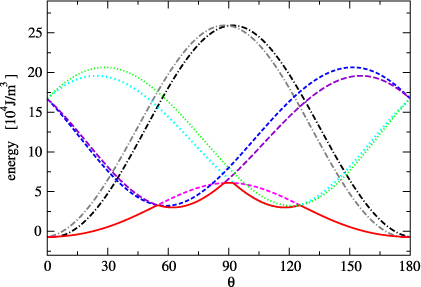
Figure 6. Anisotropy of the excited state components for magnetization in the (110) plane. The energies of individual components correspond to dotted, dashed and dashed–dotted curves, the lowest energy E0 for a given angle is emphasized by a full curve. θ is the angle, which magnetization makes with the [001] direction.
Download figure:
Standard image5. Conclusions
The discussion given above leads us to propose the following scenario for temperature dependence of the anisotropy of magnetite: above the Verwey temperature its ground state is half-metallic, possessing small magnetocrystalline anisotropy characterized by the negative K1 anisotropy constant. An excited state at energy Δ above the ground state is degenerate and its anisotropy is large with positive  . Δ depends on temperature, it is large for temperatures high above the room temperature and the excited state is almost empty. With decreasing temperature Δ is reduced and below RT the population of the excited state leads to a notable change in the temperature dependence of the anisotropy, resulting in the reversal of the sign of K1 at the spin reorientation transition. At the Verwey transition Δ becomes zero, components of the degenerate state transform to Cc crystallographic domains with considerable macroscopic distortion, the degeneracy is lifted and the positive contribution to
  (the analog ((5)) of the cubic K1) disappears.
The strong temperature dependence of Δ may be reflected in the behavior of the elastic constants, the strong temperature variation of which was reported by Ka̧kol and Kozłowski [24].
We note that a similar mechanism to that described above should also influence the magnetostriction. Indeed Brabers and Hendriks found strongly temperature-dependent magnetostriction constants in the pure and Al-substituted magnetite [25].
In conclusion, based on the experimentally determined temperatures of spin reorientation and Verwey transitions and on calculations of the anisotropy from first principles, a model explaining the anomalous temperature dependence of the magnetocrystalline anisotropy in the cubic phase of magnetite was proposed. As a by-product of the electron structure calculations the gap in the band structure of the majority spin electrons in defect-containing magnetite was calculated. This quantity could be important for eventual application of magnetite in spintronics.
Acknowledgments
This work was supported by the Grant Agency of the Czech Republic under project no. 202/08/0541, project no. 392111 of the Grant Agency of the Charles University, project MS0021620834 of the Ministry of Education of the Czech Republic and project SVV-2011-263303. The authors are grateful to Professor V A M Brabers of Einhoven University of Technology, The Netherlands, Professor J M Honig, Purdue University, USA and Professor A Kozłowski, AGH Kraków, Poland for supplying the single crystals of magnetites.