
Abstract
By exploring a simple model of a negative thermal expansion (NTE) system, we introduce a phenomenological expression to describe the temperature dependence of the pressure-induced softening in NTE structures.
Export citation and abstract BibTeX RIS
1. Introduction
Normally, materials become stiffer when compressed, as is measured by their positive first pressure derivative of the bulk modulus,  . However, some materials are recently found to show negative
  and they actually become softer on compression. This counterintuitive phenomenon called 'pressure-induced softening' has been observed in ZrW2O8 [1] and Zn(CN)2 [2, 3], and is likely to be a general feature shared among materials having negative thermal expansion (NTE) [4]. We further found that would first become more negative and then tend to zero at high temperatures [3]. Here, by exploring a simple model of NTE system, we will introduce and show that the temperature dependence of the 'pressure-induced softening' (indicated by the value of ) can indeed be described by the expression introduced in [3],

parameterized by the variables  , T0 > 0, and T1 > 0 defined in figure 1.
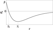
Figure 1. Schematic curve showing the variation of with temperature T according to equation (1), which defines the parameters  , T0 and T1.
Download figure:
Standard image High-resolution imageThe paper is structured as follows. A simple model of NTE system is presented with the bulk modulus (B0) and its first pressure derivative () derived for cases with and without anharmonicity. The physical meaning of the phenomenological expression (equation (1)) is then explored against the results from the model. Finally, the application of equation (1) to describe the temperature dependence of the 'pressure-induced softening' of several zeolite structures is discussed.
2. Theory and results
2.1. The model
Perhaps the simplest model to have NTE is the one shown in figure 2, where each rigid-square unit rotates against each other on heating while the unit itself is totally rigid for thermal excitation, resulting in the reduction of distance between the near square centers hence the thermal contraction of the whole system.

Figure 2. Configuration of a simple model for a NTE system. The squares are rigid units immune from thermal excitation. Different match of the arrows shows different rotational modes of the rigid units on heating.
Download figure:
Standard image High-resolution imageThe energy of such a system in an independent-object model where coupled terms are ignored (as suggested by [1, 4]) can be written as,

with

Because of the cell reduction by a factor of (1 −cosθ) due to rotation of the square with a tilting angle of θ, this term lowers the energy for compression or rotations. Erot describes the energy cost of the rotation with even powers of θ and K1, K2 > 0,

The fourth-order terms of θ in EpL and Erot are related to the anharmonicity of the thermally excited rotation modes. Est is the strain energy inside the squares under pressure p, where the bonds from the centre to the apex of the square can for example correspond to Zr/W–O bonds in ZrW2O8 or Zn–C/N bonds in Zn(CN)2.
With a partition function calculated using the energy in equation (2), the expectation value of θ2 at temperature τ = kBT is,
where the strain energy Est is independent from θ. cosθ is expanded as cosθ = 1 − θ2/2! + θ4/4! . Using a mean-field theory [5], one can approximate the fourth-order term of θ as

where the factor of 3 comes from the numerical test that 〈θ4〉 = 3〈θ2〉2, and we put 〈θ2〉≈ 4Cτ in the classical approximation with positive coefficient C (the factor of 4 is for derivation convenience). By inserting this in equation (5) and putting
one can rewrite the equation as
where c = χ1 + χ2τ /τ. Note that the positive coefficient C (see equation (6)) and hence χ2 defined by equation (7) provide a measure for the magnitude of the mode anharmonicity. We put the equilibrium cell length as unit 1 for convenience so that the pressure p and the force constants K1 as well as K2 (in equation (7)) all have energy dimensions in the model. The coefficient C has dimension of 1/energy (in equation (6)). χ1 has energy dimension and χ2 is dimensionless.
In such a model, for a small pressure p, the reduction of cell length (ΔL: length, area and volume reductions in one, two and three dimensions, respectively) at temperature τ is proportional to the expectation value 〈θ2〉τ plus the compressed strain e ≈−κp < 0 of the bonds inside the square,

with

as the compressibility of the bond that decreases on compression. a and b (in equation (10)) have dimensions of 1/energy and 1/energy2, respectively.
2.2. Temperature dependence of B0 and 
With the model being established, we can now discuss the temperature dependence of the bulk modulus (B0) and its pressure derivative (). The bulk modulus can be calculated from equation (9) as,
where we have used ∂χ1/∂p = −1 and ∂χ2/∂p = C according to equation (7).
For zero anharmonicity, when χ2 = C = 0, equation (11) becomes
with an asymptotic form of
where we have put τ = τZ + τ' with τZ a small constant representing the contribution from the quantum zero-point energy. Thus, B0 (defined as B at p = 0) with χ1 = K1 and κ = a starts as the modulus of the bond (1/κ) at zero temperature and decreases as 1/τ on heating. The schematic plot of B0(T) is shown as the dash curve in figure 3(a).
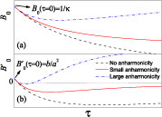
Figure 3. Temperature dependence of (a) B0 and (b) with and without anharmonicity in the rotational terms of the model.
Download figure:
Standard image High-resolution imageThe first derivative of B with respect to pressure can be calculated from equation (12) as
At zero temperature, (defined as at p = 0) with χ1 = K1 and κ = a is

which shows that the value of at zero temperature is positive and equal to the pressure derivative of the bond modulus (see equation (10)). However, will become negative on heating as shown in equation (14). It also has an asymptotic form of

meaning that tends to zero with τ→∞. The schematic plot of  is shown as the dash curve in figure 3(b).
In the case of small anharmonicity, such that C and hence χ2 are both small quantities with negligible high-order terms of O(C2) and  , the bulk modulus from equation (11) becomes
Note that B0 ≈ 1/κ at zero temperature. The value of B0 will increase linearly with τ→∞. These are shown by the solid curve in figure 3(a).
From equation (17), one can further obtain,
At zero temperature, is the same as in equation (15). However, with the anharmonic terms, the value of will tend to zero more rapidly with temperature than the one without anharmonicity. For the case of large mode anharmonicity, the value may even become positive again. These are shown by the solid and the dash-dot curves in figure 3(b) compared to the dash curve without anharmonicity.
To sum up, the value of at zero temperature is positive and equal to the pressure derivative of the modulus of the bond, b/a2 (see equation (10)). With elevated temperature, becomes negative and tends to zero with τ→∞ if the mode anharmonicity is not large. Thus, in both cases with and without anharmonicity, a phenomenological expression as illustrated in figure 1 is a good yet simple description for the temperature dependence of . At zero temperature this form gives a positive value , and at high temperature this expression shows an asymptotic behaviour similar to −exp(−T) that tends to zero.
2.3. Parameters in the phenomenological expression
Besides its simplicity, the advantage of the phenomenological expression of equation (1) is that its three variables can be assigned with physical meanings. is the value of at zero temperature. It is the pressure derivative of the bond modulus. T0 is the temperature at which the value of drops to zero, corresponding to τ0 that makes equation (18) equal to zero,

Note that with zero anharmonicity, i.e. C = K2 = 0, T0 is equal to the solution of equation (14) as expected. In the model, since the bond modulus is 1/κ = 1/(a − bp), 1/a is its value at zero pressure and equal to the force constant k of the bond potential. Thus, one may rewrite equation (19) as

where the ratio between the force constants of the rotational term of the rigid unit modes (RUMs) and the bond term, K1/k, gives a measure of the relative stiffness of the two. The force constant K1 can correspond to a mean frequency of the RUMs that have significant negative mode Grüneisen parameters leading to NTE of the system. Therefore, the value of T0 is akin to the flexibility of the structure and the characteristic frequency of the RUMs; more structure flexibility and smaller RUM frequency would result in a smaller value of T0. It is also clear that T0 will increase due to the anharmonic term measured by C.
T1 corresponds to the temperature at which reaches its minimum. From equation (18) one can obtain
which shows that T1 is also determined by the flexibility of the structure and the characteristic frequency of the RUMs. By comparison with equation (20), we can see that the value of T1 should be larger than two times T0, given that the anharmonic coefficient C is a small quantity.
Note that, other than the anharmonic terms (involving C) in T0 and T1, the dominant terms in these two quantities are related to the value of which is material-dependent. This makes the value of T0 or T1 not such a good indicator for comparing anharmonicity between different materials. To cancel the dependence of the dominant term on , the difference between T1 and two times T0 is calculated,

This value is positive and shows how fast can reach its minimum on heating and provides a better measurement of the anharmonicity of the system, i.e. the larger the anharmonicity C, the smaller the value of T1 − 2T0, as shown in figure 3.
3. Discussion
3.1. of some zeolite structures

As a demonstration, we now apply the phenomenological expression of equation (1) to some silicious zeolite structures that show isotropic NTE [4], including FAU, KFI, LTA and TSC [6]. We have carried out molecular dynamics (MD) simulations for the structures in [4] using DL_POLY [7], with O–O, Si–O and Si–Si interactions described by Coulomb interactions and Buckingham potentials ϕ(r) of the form

where rij is the distance between two atoms of type i and j. The parameters Aij, ρij and Cij for each atom pair type are taken from the force field of Tsuneyuki [8]. To obtain the values of at different temperatures, we used the third-order Birch–Murnaghan equation of state (EoS) [9] to fit to the isotherms of these structures from the MD, as shown in figure 4 for T = 1 K. Fitting to the isotherms at other temperatures from the simulations and testing the calculated results against the available experiments can be found in [4].

Figure 4. Fitting to the isotherms at 1 K from the MD simulations using the third-order Birch–Murnaghan EoS.
Download figure:
Standard image High-resolution image3.2. Apply the phenomenological expression to the zeolite structures
According to the simple model in section 2, T0 and T1 in the phenomenological expression are akin to the (rotation) modes that lead to NTE of the system. To have an idea of how these modes exist in the zeolite structures we have studied, the density of states (DoS) and the Grüneisen parameters were calculated by harmonic lattice dynamics using GULP [10] with the same potential model as in the MD. As shown in figure 5, where the DoS of each structure is coloured according to the values of Grüneisen parameters, all the modes with significant negative Grüneisen parameters hence most relevant to NTE of the structure are below 3.0 THz (∼150 K). Thus, to reduce the error introduced by the deviation of the classical simulation from the real quantum picture at low temperatures [11], we will only use the data points of at temperature beyond 200 K when any mode with significant negative Grüneisen parameter has been well excited.
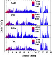
Figure 5. Calculated density of states (DoS) for each zeolite structure using GULP [10] with the same potential model used in the MD. Each DoS was coloured according to the values of Grüneisen parameters to highlight the most important modes that have the most negative Grüneisen parameters. The dotted vertical line shows the value of 1.5 THz. Modes with frequencies below this value account for 70% of the total number of modes having negative Grüneisen parameters.
Download figure:
Standard image High-resolution imageThe zero-temperature value of , i.e. the value of , was obtained from the harmonic lattice calculations. Figure 6 shows the fitted temperature dependence of for each zeolite using the phenomenological expression (equation (1)). The fitted values of variables T0 and T1 are listed in table 1. Although the data points below 200 K were not used in the fitting, they show consistent trend with the curves.

Figure 6. Using the phenomenological expression of equation (1) to fit to the data beyond 200 K (full circle with error bar) for the studied zeolite structure with two variables T0 and T1. The value of (zero-temperature ) was calculated in Harmonic lattice dynamics using GULP [10]. Data points from 1 to 100 K (open circles) are also shown with similar trend to the fitted curve. The dotted lines show positions of the zero value.
Download figure:
Standard image High-resolution image
Table 1.
Values of T0 and T1 for the zeolite structures from fitting to the data using the phenomenological expression of equation (1). The value of at zero temperature, i.e. , for each structure was calculated using harmonic lattice dynamics.
| Zeolite | |
T0 (K) | T1 (K) | T1 − 2T0 (K) |
|---|---|---|---|---|
| FAU | 2.4 | 89(16) | 493(98) | 314(114) |
| KFI | 2.6 | 84(12) | 604(113) | 437(125) |
| LTA | 3.0 | 17(2) | 260(25) | 225(27) |
| TSC | 0.5 | 12(2) | 384(59) | 361(61) |
From figure 5, we found that, among all the modes that have negative Grüneisen parameters, those with frequencies no larger than 1.5 THz (indicated by the dotted line) account for 70% of the total number of modes and these modes also constituent 70% NTE of the structure in terms of the value of the overall Grüneisen parameter. It is clear that the fitted T0 of the zeolites agrees with this characteristic frequency (1.5 THz ≈ 75 K). The values of T1 − 2T0 of the zeolites indicate that LTA should have larger anharmonicity than TSC and FAU should have larger anharmonicity compared to KFI.
Because is a second-order quantity, it is very sensitive to errors in isotherm data, which gives us a challenge to directly measure its temperature dependence accurately, especially for low-temperature points [3]. However, by using the proposed phenomenological expression of equation (1), one is able to have access to the temperature dependency of of NTE materials at low temperatures, with the zero-temperature value easily calculated from a reliable theoretic model and the data points at high temperatures where the experimental error becomes acceptable.
Acknowledgments
We gratefully acknowledge financial support from the CISS of Cambridge Overseas Trust (HF). MD simulations were performed using the CamGrid high-throughput environment of the University of Cambridge. The interatomic potential was developed through our membership of the UK HPC Materials Chemistry Consortium, funded by EPSRC (EP/F067496), using the HECToR national high-performance computing service provided by UoE HPCx Ltd at the University of Edinburgh, Cray Inc. and NAG Ltd, and funded by the Office of Science and Technology through EPSRC's High End Computing programme.