
Abstract
Systems with short-range attractive and long-range repulsive interactions are able to form mesophases at sufficiently low temperatures. In two dimensions, such mesophases emerge as clusters, stripes or bubbles. Using extensive Monte Carlo simulations we investigate the static and the dynamic properties of such a cluster-forming system over a broad temperature range and for different densities. Via the static properties we analyse how ordering into close packed configurations sets in both at the level of the particles as well as at the level of the clusters. The dynamic properties provide information on how, at low temperature, the motion of individual particles is influenced by the dynamic slowing down of the clusters. Finally, we discuss the different diffusion mechanisms at play at low and intermediate densities.
Export citation and abstract BibTeX RIS

Original content from this work may be used under the terms of the Creative Commons Attribution 3.0 licence. Any further distribution of this work must maintain attribution to the author(s) and the title of the work, journal citation and DOI.
1. Introduction
When cooled at sufficiently low temperatures, particles whose interactions are given by a repulsive core region with an adjacent tail, composed of a short-range attraction and a long-range repulsion, are able to form so-called mesophases. While in two dimensions these phases comprise clusters, stripes and bubbles, they are considerably more complex in three dimensions, where the emergence of spherical clusters, ordered arrangements of cylinders or layers have been reported. The formation of such complex phases is quite surprising as it occurs for systems with spherically symmetric interactions [1].
Indeed, a considerable amount of effort has been dedicated to the theoretical study of such phases [2–14]. Most of these investigations were based on a standard interaction model that mimics the two aforementioned, specified features via a simple functional form. Originally introduced by Sear et al [15], this interaction potential consists of a hard core region plus a linear combination of two exponential functions: as the prefactors of these contributions have opposite signs, they represent the two characteristic parts of the interactions (see equation (1)). Experimental evidence for the formation of these microphases has also been given, for both two [16–20] and three [21–24] dimensional systems.
The overwhelming majority of the theoretical investigations on these systems was dedicated to the static properties. In this contribution, we present a systematic study of the dynamic properties of a system where particles interact via a short-range attractive, long-range repulsive potential; to be more specific, we focus on the cluster phase of the two dimensional model studied in [2, 3, 5, 15], in the regime of small and intermediate densities and at low temperatures. Our investigations are based on extensive Monte Carlo simulations along three selected isochores. We gradually decrease the temperature and characterize the dynamic slowing down of the fluid. By using a suitable cluster identification algorithm we are able to calculate the static and the dynamic properties of both the individual particles as well as of the clusters (specified by their centers-of-mass).
With the help of the static properties, we analyse how the ordering of the system sets in as we decrease the temperature. On one side, we observe formation of an ordered, hexagonal cluster pattern; on the other side, we observe the emergence of local close-packed arrangements of the particles within the clusters. Our data indicate that these ordering processes are independent of one another and have subtle signatures in both the thermodynamic (i.e. specific heat) and dynamic properties of the system.
The dynamic properties, calculated separately for the cluster and for the individual particles, comprise the respective mean squared displacements, the diffusion coefficients, and the intermediate scattering functions. We observe that both for the individual particles as well as for the clusters a subdiffusive behaviour can be observed, which occurs at length scales that correspond to the average cluster size. The intermediate scatting functions provide evidence of a two step relaxation of the dynamics of the individual particles, with typical relaxation times that increase mildly as the temperature is lowered. The cluster intermediate scattering functions display instead a simple, single-step relaxation mechanism.
We also observe qualitative variations of the dynamics as a function of density. At intermediate densities, particles can diffuse at low temperature by migrating from cluster to cluster, even when the cluster structure is essentially frozen. At low density, by contrast, the system assembles into relatively rigid clusters, which diffuse slowly and do not show signatures of global ordering on our observation time scale. Our results thus suggests that, at low density, the system may form a 'cluster glass' [39] when cooled to even lower temperature.
The manuscript is organized as follows: in the subsequent sections 2 and 3 we present our model and provide details about the Monte Carlo simulation and our cluster identification analysis. Section 4 is dedicated to the results: we start with an overview over the general properties of the clusters (in terms of size and their size distribution), we then proceed to the static structural properties of the clusters and then discuss the thermal properties of the aggregates (in terms of the specific heat); the last section is dedicated to the dynamic properties of the individual particles and of the clusters and their interrelation. The manuscript is closed with a summary.
2. Model
In our two dimensional system the particles are assumed to interact via the following spherically symmetric potential  , first introduced by Sear et al [15]:
This interaction, which can be viewed as an effective potential of a realistic colloidal system, is characterized by a hard core region (specified via the diameter σ); for distances larger than σ the interaction is given by a linear combination of a short-range attraction, quantified via the range Ra and strength  , and a long-range repulsion, specified via the range Rr and strength
  .
.
The system is characterized by a temperature T, with  , kB being the Boltzmann constant; for the reduced temperature units we use the arbitrary scale introduced in [2], i.e. for
  and for
  we set
  . The density of the system is given by ρ (with its reduced counterpart
  ); further we use the following reduced units
  and
and  . For the sake of a simplified notation, we will drop the asterisk henceforward.
Throughout this work we use  ,
,  , and
, and  . Figure 1 depicts the interaction potential
  for this particular set of parameters.

Figure 1. Interaction potential  as a function of r (see equation (1)) as used in the present work for numerical parameters specified in the text.
Download figure:
Standard image High-resolution image3. Methods
3.1. Monte Carlo simulations
The static and dynamic properties of the system are investigated by means of extensive Monte Carlo (MC) simulations [25, 26], which we perform in the two-dimensional NVT ensemble. We simulate N =4000 particles in a quadratic simulation cell with periodic boundary conditions. In an effort to enhance the efficiency of our simulations, we limit the positions of the particles to discrete lattice sites: this is achieved by dividing our square-shaped simulation box (with box lengths L ranging—depending on the densities considered—from 141.42 to 200.00) into  equally sized squares [27, 28]. The efficiency of our simulations is further improved by the use of cell lists. The maximum spatial displacement,
  , is set to ±0.15 and the cutoff radius of the potential is chosen to be
  .
.
Note that the choice of a relatively small particle displacement  enables us to interpret the MC dynamics as mimicking qualitatively the Brownian motion of colloidal particles in a solvent (overdamped dynamics). We point out, however, that establishing a precise correspondence between MC and Brownian dynamics is a delicate issue [29, 31] and that different mapping schemes between Monte Carlo and molecular dynamics type of simulations are available in literature (see, e.g. [30]).
We simulated systems at three different densities, namely  ,
,  and
and  . For each of these three cases, we performed a first set of MC simulations at a temperature of T =1.30. Then we progressively lowered the temperature of the system according to the following quenching protocol: the final configuration of the higher temperature run is used as an initial particle arrangement of the subsequent simulation at a lower temperature. The equilibration run is then followed by a production run during which we measure static and dynamic observables. An overview of the state points we investigated by repeated application of this procedure is shown in figure 2.
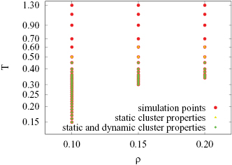
Figure 2. Overview over states investigated in this study via MC simulations in the  plane (note the logarithmic scale along the temperature axis). State points for which static or static and dynamic cluster properties have been investigated are specified via an additional green/yellow colour code (as specified).
Download figure:
Standard image High-resolution imageFor each of the three densities, ten independent quenches are performed: each of them is started at T = 1.30 from a random initial configuration. The duration of the simulation is increased progressively with decreasing temperature, i.e. from 5000 MC-sweeps at T = 1.30 to 42 500 000 MC-sweeps for the lowest investigated temperatures (i.e. for T = 0.15 and  ), where a MC-sweep consists of N attempted MC-moves. For each production run, 5000 particle configurations were collected. To investigate dynamic processes on short time-scales, additional, shorter simulations were performed, during which the particle properties were stored in much shorter time intervals.
3.2. Cluster
We identify clusters in the system using the following proximity criterion: a particle is considered to belong to a particular cluster if its distance d to another particle within the same cluster is smaller than the so-called cluster-distance parameter, dcl, for which we have assumed the value  . In the present work we consider a set of particles that fulfill the cluster criterion as a cluster, if it consists of at least five particles. Smaller sets of particles are not considered as clusters and are categorized instead as 'free' particles.
Once all clusters have been identified for a given particle configuration, we calculate their static and dynamic properties from their center-of-mass positions. The computation of the dynamic properties of the clusters is done by tracking the evolution of individual clusters over several MC sweeps. Here, we assume that the distance over which a cluster can propagate during one MC sweep is smaller than half the typical distance between two clusters; this assumption has been verified in our study. During the simulation, clusters may (i) split, (ii) merge, (iii) dissolve into free particles, or (iv) emerge from isolated particles; these events delimit the time window over which a cluster retains its identity, see [32] for more details. Time-dependent correlation functions of individual clusters, such as the mean squared displacement or the self intermediate scattering functions (see section 4.4), are evaluated over time windows during which individual clusters retain their identity.
4. Results
In the presentation of our results we first focus on some general properties of the clusters; we then proceed to their static structure and compare these data with the corresponding results of the individual particles. Next, we analyze the thermal properties of the system and eventually we discuss the dynamic properties of the clusters along with those the isolated particles.
4.1. General properties of the clusters
We start our discussion by analyzing the distribution of the size of the clusters in the system and how it varies with temperature. The size of a cluster is defined here as the number n of particles that belong to it.
In figure 3 we show representative results for the cluster size distribution at a density  . At high temperature, the distribution is strongly peaked at n = 0 and decays monotonically with n. Thus most particles in the system are free and large clusters are only formed occasionally. Below a certain threshold temperature
  , however, the distribution becomes bimodal and develops an additional maximum, which indicates the formation of stable, well-defined clusters. This feature provides us with a first criterion to identify the transition to a cluster phase. The behavior at the two other densities we investigated (i.e.
  and
and  ) is qualitatively similar. We found that the clustering temperature increases with increasing density and is
  at
at  and
and  at
at  .
.
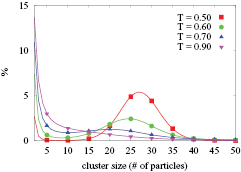
Figure 3. Distribution of the cluster size (in terms of number of particles) for our system calculated at a density  at various temperatures (as labeled).
Download figure:
Standard image High-resolution imageFigure 4 displays the average cluster size as a function of the temperature T. We observe that the cluster size shifts to larger values with increasing density and increases by decreasing temperature. At temperatures well below the clustering temperature, however, the cluster size eventually becomes constant. This suggests that the internal cluster structure freezes at sufficiently low temperature.
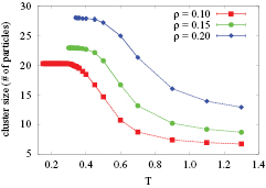
Figure 4. Cluster size (in terms of number of particles pertaining to a cluster) as a function of T for the three investigated densities ( ,
,  and
and  ; as labeled). For temperatures below the clustering temperature (see table 1) the symbols are connected by a continuous line, while above this temperature a broken line is used as a guide for the eyes.
Download figure:
Standard image High-resolution imageTable 1. Clustering temperatures Tcl, ordering temperatures of the individual particles and of the clusters,  and
and  (see text for definition) for the three studied densities.
| ρ | Tcl |  |
 |
|---|---|---|---|
| 0.10 | ≈0.5 |  |
— |
| 0.15 | ≈0.6 |  |
 |
| 0.20 | ≈0.7 |  |
 |
Note: No estimate for  could be obtained for
  .
.
As an additional measure of the typical extent of a cluster, we introduce the radius of gyration [3]
with n being the number of particles pertaining to a given cluster, and dij being the distance between particles i and j of this cluster. Figure 5 shows Rg as a function of the temperature and for all three values of density investigated.

Figure 5. Radius of gyration, Rg, as a function of temperature for the three densities investigated ( ,
,  and
and  ; as labeled). For temperatures below the clustering temperature (see table 1) the symbols are connected by a continuous line, while above this temperature a broken line is used as a guide for the eyes.
Download figure:
Standard image High-resolution imageFor a fixed density, Rg first increases with decreasing temperature and attains its maximum value close to the clustering temperature. From the coincidence of these two temperature values we conclude that the above introduced criterion based on the cluster-size distribution is appropriate. As we further decrease the temperature below this threshold value, Rg decays monotonously. In this regime, the cluster occupation number is either constant or slowly increasing (see figure 4), but the typical spatial extent of a clusters decreases due to the reduced thermal motion of the particles.
Finally, we show in figure 6 the percentage of free particles, i.e. single particles and/or clusters with a size less than five particles, as a function of T. As expected, this number shows a pronounced increase at T-values close to the clustering temperature. Interestingly clusters start to dissolve when the amount of free particles reaches a value of ∼12%, irrespective of the density ρ.
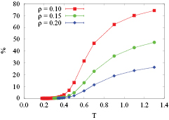
Figure 6. Percentage of free particles in the system (see text) as a function of temperature for the three investigated densities ( ,
,  and
and  ; as labeled). For temperatures below the clustering temperature (see table 1) the symbols are connected by a continuous line, while above this temperature a broken line is used as a guide for the eyes.
Download figure:
Standard image High-resolution image4.2. Structural properties of the clusters
In this section we discuss the static structure of the clusters and compare it with the corresponding results for the individual particles.
As the temperature is lowered at a fixed density, we find clear signatures of ordering in the system, both at the level of individual particles and of the clusters. To illustrate these features, we show in figure 7 the radial distribution function g(r) of the particles and of the clusters, as obtained from their centers-of-mass, for the state point  , T = 0.35. The two panels of the figure show data for either the small- (top panel) or the large-distance (bottom panel) range. Results for other combinations of density and temperature can be found in [32].
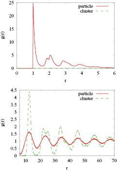
Figure 7. Radial distribution function, g(r), of the particles and of the clusters (as labeled) calculated at a density  and at a temperature T = 0.35. Upper panel: g(r) for r-values up to 6, lower part: g(r) for r-values up to 70. Note the different vertical scales in the two panels.
Download figure:
Standard image High-resolution imageFor small distances (i.e. up to  ) the radial distribution function of the particles shows a characteristic pattern of peaks, reflecting the close-packed, internal structure that the particles form within the clusters. This packing originates from the balance between the short-range attraction between the particles and the repulsion that each cluster experiences from the neighbouring clusters. The data for this specific state point display a pronounced splitting of the second peak at
  and an additional shoulder at
  , which provides evidence for regular arrangements within the cluster: these two peaks, along with the position of the main peak, are consistent with the formation of an internal hexagonal structure, which becomes also evident from visual inspection of simulation snapshots [32]. The splitting was considered in [3] as a precursor of freezing within the clusters.
By contrast, the cluster-based g(r) vanishes in this range of distances: due to the accumulated long-range repulsion of the particles that form these aggregates, the clusters repel each other on these length scales. The radial distribution function between the clusters shows its first peak only at a distance  (see bottom panel of figure 7), followed by two peaks at
  and
and  . These two peaks do not only have the same relative positions with respect to the location of the main maximum; they also display similar splitting as the corresponding maxima in the particle g(r). We therefore conclude that, at least for this state point, also the clusters themselves arrange in a regular, hexagonal lattice, as confirmed by visual inspection of simulation generated snapshots. Similar observations were made for the other densities investigated and for T-values up to the respective clustering temperatures.
In the following we will use the emergence of this characteristic peak pattern as an estimate of the freezing temperature of the particles,  , and of the clusters,
  , respectively. The corresponding values (where available) are collected in table 1. We observe that the values of
  depend only weakly of ρ. By contrast, the freezing temperature of the clusters,
  , displays a strong density-dependence. For
  , an estimate for this temperature value is rather difficult to obtain: at this density, we could not observe the characteristic features of the first three main peaks in the cluster g(r) in the investigated temperature range. Thus we conclude that for
  clusters do not freeze, at least in the temperature range that was accessible to our simulations. Despite the relatively large error bars, our data suggest that clusters may, depending on temperature, first arrange into an hexagonal lattice, with their internal structure being still disordered, or freeze internally while remaining in a fluid state. This, in turn, indicates that freezing of the clusters and freezing within the cluster are as two independent physical processes.
In an effort to assess on a quantitative level the degree of ordering of the clusters, we use here two measures based on the conventional hexagonal bond order parameter  [33–36]. In this way we will be able to quantify the transition of the system in to an hexagonally ordered cluster phase with more precision.
The hexagonal bond order parameter of a single cluster in the surrounding of its neighboring clusters, ![$ \Psi _{6}^{[1]}$](https://content.cld.iop.org/journals/0953-8984/28/41/414015/revision1/cmaa277aieqn070.gif) , can be computed via
, can be computed via
with M being the number of the nearest neighbors and  being the angle between the (arbitrarily chosen) x-axis and the vector from the center cluster to the nearest neighbor cluster m.
 ![$ \Psi _{6}^{[1]}$](https://content.cld.iop.org/journals/0953-8984/28/41/414015/revision1/cmaa277aieqn072.gif) is 1 for a perfect hexagonal cluster arrangement, while it vanishes in the case of random arrangements.
is 1 for a perfect hexagonal cluster arrangement, while it vanishes in the case of random arrangements.
The average hexagonal bond order parameter,  , is obtained by averaging both over all clusters of the system and along the simulation run; it is calculated via
here J is the number of configurations retained for the average, Nj the number of clusters identified in simulation snapshot j and Mj, n is the number of nearest neighbors of cluster n in snapshot j.  in equation (4) denotes the angle between the (arbitrarily chosen) x-axis and the vector connecting the centers of mass of the central cluster n with its nearest neighbor m in simulation snapshot j.
The results of  are shown in figure 8 as function of temperature for the three densities investigated in this study. For
  and
and  the hexagonal bond order parameter
  increased significantly with decreasing temperature: eventually, for the lowest temperatures investigated,
  attains values of up to ∼0.7–0.8 for these two ρ-values. This abrupt change in
  occurs, however, already at a temperature that is higher than the freezing temperature of the clusters, predicted via the radial distribution functions, see table 1. By contrast, for
  ,
,  attains values that hardly exceed 0.2. These observations support the previous claim that the clusters do not freeze for densities
  , at least in the investigated temperature range.
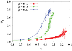
Figure 8. Hexagonal bond order parameter,  , as defined in equation (4) as a function of the temperature for the three investigated densities (
 ,
,  and
and  ; as labeled).
Download figure:
Standard image High-resolution imageIn figure 9 we show typical snapshots of the clusters as obtained in the simulation. Circles represent the clusters' centers-of-mass (symbols are not drawn to scale) and are color coded by the respective hexagonal bond order parameter ![$ \Psi _{6}^{[1]}$](https://content.cld.iop.org/journals/0953-8984/28/41/414015/revision1/cmaa277aieqn088.gif) . Results are shown for
. Results are shown for  at four different temperatures.
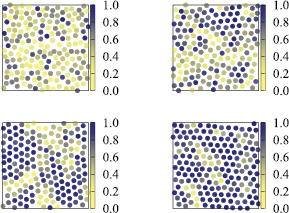
Figure 9. Hexagonal bond order parameter, ![$ \Psi _{6}^{[1]}$](https://content.cld.iop.org/journals/0953-8984/28/41/414015/revision1/cmaa277aieqn090.gif) , as defined in equation (3) for the individual clusters observed in simulation snapshots; these were taken for a system of density
, as defined in equation (3) for the individual clusters observed in simulation snapshots; these were taken for a system of density  and for different temperatures (from top left to bottom right: T = 0.50, T = 0.40, T = 0.35 and T = 0.30). The colour codes are shown on the right hand sides of the panels. The symbols representing the clusters are not drawn to scale of the actual cluster.
Download figure:
Standard image High-resolution imageAt the highest temperature, T = 0.50, we observe mainly clusters with low hexagonal bond-order parameter ![$ \Psi _{6}^{[1]}$](https://content.cld.iop.org/journals/0953-8984/28/41/414015/revision1/cmaa277aieqn092.gif) . Only a small fraction of clusters form perfect hexagonal local structures. As we decrease the temperature, hexagonal clusters tend to aggregate forming 'islands' that grow rapidly by decreasing T, see panels corresponding to T = 0.40 and T = 0.35. At this latter temperature, already about half of the clusters are characterized by an hexagonal bond order parameter that exceeds 0.7. Finally, at the lowest temperature T = 0.30 most of the clusters are characterized by a perfect hexagonal surrounding; these cluster crystalline regions, where the order parameter assumes values within the range
. Only a small fraction of clusters form perfect hexagonal local structures. As we decrease the temperature, hexagonal clusters tend to aggregate forming 'islands' that grow rapidly by decreasing T, see panels corresponding to T = 0.40 and T = 0.35. At this latter temperature, already about half of the clusters are characterized by an hexagonal bond order parameter that exceeds 0.7. Finally, at the lowest temperature T = 0.30 most of the clusters are characterized by a perfect hexagonal surrounding; these cluster crystalline regions, where the order parameter assumes values within the range ![$0.3\leqslant \Psi _{6}^{[1]}\leqslant 0.70$](https://content.cld.iop.org/journals/0953-8984/28/41/414015/revision1/cmaa277aieqn093.gif) , are intersparsed with mobile defects, which we tentatively associate to the size dispersity of the clusters.
, are intersparsed with mobile defects, which we tentatively associate to the size dispersity of the clusters.
At a density  we found a similar behavior but the growth of the high-
![$ \Psi _{6}^{[1]}$](https://content.cld.iop.org/journals/0953-8984/28/41/414015/revision1/cmaa277aieqn095.gif) cluster islands sets in at a considerably higher temperature. By contrast, at
cluster islands sets in at a considerably higher temperature. By contrast, at  , less than half of the clusters are characterized by order parameters with
 ![$ \Psi _{6}^{[1]}\geqslant 0.7$](https://content.cld.iop.org/journals/0953-8984/28/41/414015/revision1/cmaa277aieqn097.gif) , even at the lowest investigated temperature.
, even at the lowest investigated temperature.
4.3. Thermal properties of the clusters
We now inspect the thermal properties of the system for signatures of the various structural transitions (or crossovers) identified in the previous section. To this end, we calculate the excess specific heat,  via
via
with  being the excess energy of the system. The above derivative is approximated by the centered difference formula.
In figure 10 we show the excess specific heat per particle,  , as a function of temperature for the three investigated densities. For reference, we also display for the data obtained by Imperio and Reatto [3] at a density
  . The two sets of data are found to be in good agreement.

Figure 10. Excess specific heat per particle,  , as a function of the temperature for the three investigated densities (
 ,
,  and
and  ; as labeled). For reference, the corresponding
  -data as obtained by Imperio and Reatto [3] are shown.
Download figure:
Standard image High-resolution imageAs already argued in [3], the main peak in the excess specific heat (for  at a temperature
  ) is due to the latent heat involved in the formation of the microphases (i.e. the clusters) from the homogeneous fluid phase. Similar peaks, albeit smaller in their amplitude can be observed for the other two densities (i.e.
  and
and  ). The position of the main peaks shifts to higher temperature with increasing density. The temperatures at which these peaks occur peaks are in good agreement with the clustering temperatures determined in section 4.1.
For all investigated densities, the specific heat curves show an additional small local maximum/shoulder for  . Even though these features are difficult to resolve, their positions coincide within reasonable accuracy with the temperatures where the particles inside the clusters freeze into a hexagonally close packed structure (see table 1). Imperio and Reatto [3] gave a similar interpretation to a similar secondary peak peak observed in this system at
  . We point out, however, that it is difficult to clearly identify the origin of these low temperature features.
4.4. Dynamic properties
We now discuss the dynamic properties of the clusters and establish a connection with the dynamics of individual particles. We recall that we use a MC sweep as a time unit.
4.4.1. Mean squared displacement.
We start off with the mean squared displacement (MSD),  , defined either for particles and clusters as

 denotes the particle (or cluster center-of-mass) position at time t. The thermal average
  is carried out over initial times t = 0. Additionally, it is convenient to calculate the logarithmic derivative of
  with respect to time
This quantity helps us to identify the type of motion that particles or clusters realize. For a ballistic motion, z(t) = 2, while for a diffusive particle propagation z(t) = 1. Values between 0 and 1 indicate subdiffusive behavior.
In the top panel of figure 11 we display the MSD of the individual particles for a system of density  at three temperatures below the clustering temperature. In the bottom panel, we show the corresponding z(t)-curves. Since the microscopic dynamics is stochastic, the motion of the particles at short times is purely diffusive. At intermediate times, however, we observe relatively strong deviations from the diffusive behaviour, as witnessed by two pronounced minima in z(t). These deviations become stronger with decreasing temperature, with z(t) attaining values as small as 0.5 at the lowest temperatures. Thus, in these intermediate time ranges the dynamics of the system is considerably slowed down. Diffusive motion is eventually recovered at long times, except for the lowest investigated temperature, at which the particles' motion is very slow on the simulation time scale.
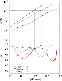
Figure 11. MSD (top panel) and z(t) (bottom panel) as functions of t of the individual particles for a system with  and at three different temperatures below the clustering temperature (as labeled).
Download figure:
Standard image High-resolution imageBy projecting the respective positions of the minima in z(t) to the top panel we can identify the typical length-scales associated to the slowing down of the particles' dynamics. The first set of minima corresponds to MSD values in the range  , thus to displacements that are small compared to the typical interparticle separation. By contrast, the second set of minima, whose locations cover three decades in time, corresponds to MSD-values of about 20 and which are essentially temperature-independent. This corresponds to an average displacement of
  , which is of the order of the radius of gyration, Rg. Thus we attribute the second minimum in z(t) and the ensuing slowing down of the dynamics to the attractive forces preventing particles from leaving the cluster and which ultimately hold the cluster together.
Analysis of the MSD at higher density shows the length scales associated to the cluster slowing down grows only weakly with increasing density, see table 2. By increasing the density at constant temperature, however, the position of the second minimum in z(t) shifts to larger t-values; this effect is due to the increase in cluster size with increasing density: the increasingly larger surrounding clusters exert a stronger repulsion on the particles of a tagged cluster, reducing thereby their MSD [32].
Table 2. Time-range,  , of the occurrence of the second minima in z(t) and corresponding range in the MSDs,
  , for the individual particles (index 'pt'; columns two and three) and for the clusters (index 'cl'; columns four and five) for the three densities investigated; the indicated ranges reflect the temperature-dependence of these quantities.
| ρ |  |
 |
 |
 |
|---|---|---|---|---|
| 0.10 | 1.0 104–8.0 106 | 1.5 101–1.9 101 | 4.8 104– 7.1 106 | 8.1 100–1.1 101 |
| 0.15 | 1.4 104–1.8 105 | 1.4 101–2.0 101 | 5.9 104– 1.3 106 | 5.8 100– 7.6 100 |
| 0.20 | 2.2 104–1.3 105 | 1.6 101– 2.1 101 | 2.2 105– 6.0 105 | 3.8 100–6.4 100 |
To corroborate our analysis, we now evaluate the MSD from the clusters' center-of-mass positions. The corresponding data and related local exponents z(t) are shown in figure 12 for  at temperatures below the clustering temperature (i.e. for
  ). For all these temperatures, the cluster-based z(t)-curves display a relatively pronounced first minimum, whose position lies in the range of up to 100 time units. As the corresponding cluster-MSD values are well below 10−2, these effects are not of particular relevance. The second minima in the cluster-z(t) are located in the range
  (T = 0.45) to
  (T = 0.15), spanning thus more than two decades in time. Again, if we trace back from the positions of these minima the corresponding values of the cluster-MSD (ranging—essentially independent of the temperature—in the narrow interval
  ), we observe that these MSD-values correspond to an average cluster displacement of about
  .
.
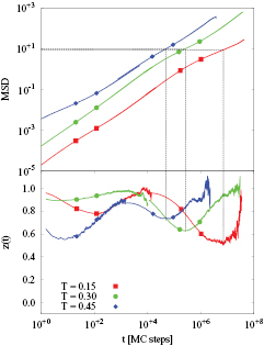
Figure 12. MSD (top panel) and z(t) (bottom panel) as functions of t of the clusters for a system with  and at three different temperatures below the clustering temperature (as labeled).
Download figure:
Standard image High-resolution imageTo conclude this section, we briefly proceed to the other densities, i.e.  and
and  , focusing on the positions of the second minima in z(t). The temperature-dependent time-range of their occurrence and the corresponding range in the cluster-MSDs are compiled for all three densities investigated in table 2. In contrast to the corresponding individual particle level (see table 2), we observe that the range of MSDs where the dynamic slowing down of the clusters occurs shows a pronounced density-dependence. We observe a shift to larger MSD-values as the density decreases: for high densities the clusters are considerably larger, restricting thereby to a larger extent the mobility of the neighbouring cluster than this is the case at low densities.
4.4.2. Diffusion coefficients.
The diffusion coefficient, D, can be extracted from the MSD via the Einstein relation at sufficiently long times,
In figure 13 we present the diffusion coefficients of the clusters,  , and the diffusion coefficient of the individual particles,
  , as functions of the temperature for the densities
  (top panel) and
  (bottom panel). We choose an Arrhenius representation (
 versus 1/T) to account for the broad dynamic range covered in our simulations. Note that we only calculate the cluster diffusion coefficient for temperatures below the clustering temperature Tcl, at which clusters become well-defined.

Figure 13. Diffusion coefficients, D, of clusters and of the individual particles (as labels) as functions of the inverse temperature (scale in the bottom) and of the temperature (scale at the top) for densities  (top panel) and
  (bottom panel). Note the logarithmic scale used for D.
Download figure:
Standard image High-resolution imageThe motion of the particles slows down progressively as the system is cooled down from high temperature. For all studied densities, the temperature dependence of the diffusion coefficients shows a first broad crossover around the clustering temperature Tcl, below which D slows down considerably and roughly follows the Arrhenius law  , where E is an 'effective' activation energy. Note that, at the temperatures at which stable clusters first appear, their diffusion coefficient is about two orders of magnitude smaller than the one of the particles, irrespective of density.
As the temperature is decreased further, however, the data at low and high densities show different patterns. For  , the diffusion coefficients of the particles and for the clusters tend to converge and become identical for temperatures below
  . This indicates that for temperatures below this threshold value, clusters behave as 'rigid' objects and the diffusion of the particles is dictated by the slow diffusion of the clusters. We note that in this low temperature regime, the temperature dependence of the diffusion coefficients is milder than Arrhenius, which suggests that the relaxation of the clusters proceeds through mechanisms different from the ones usually encountered in conventional glassy systems [38], e.g. activated dynamics.
For  instead, both diffusion coefficients decrease with decreasing temperature, but their ratios remain nearly constant below Tcl. In this regime, the temperature dependence of both Dcl and Dpt is well described by the Arrhenius laws with very similar effective activation energies. We speculate that the clusters' diffusion at low temperature is related to the motion of 'defects' in a nearly frozen cluster crystalline structure, see figure 8. At the lowest investigated temperatures, at which the motion of the clusters appears essentially arrested on the simulation time scale, the particles still display a residual diffusion, which we tentatively attribute to migration from cluster to cluster. Similar considerations hold for
  (data not shown).
In figure 14 we show Dcl as a function of 1/T for all investigated densities. We see that density exerts a strong effect on the cluster dynamics: Dcl drops faster as density increases, even when the temperature is rescaled by the density dependent T cl. These observations are consistent with the structural analysis presented in section 4.2, where we concluded that local ordering was much less pronounced in the low density system. In this latter case, the dynamics of the system can be characterized as a fluid of slowly diffusing and 'rigid' clusters. Note, however, that the particle diffusion depends strongly on density only at low temperature [32].
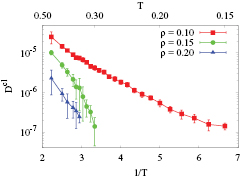
Figure 14. Diffusion coefficients of the clusters,  , as functions of the inverse temperature (scale in the bottom) and of the temperature (scale at the top), calculated for different densities (as labeled).
Download figure:
Standard image High-resolution image4.4.3. The intermediate scattering functions.
To characterize the relaxation of density fluctuations at intermediate length scales, we evaluate the total intermediate scattering function (ISF),  . This is defined as the time correlation function of the Fourier transform of the particle at a given wave-vector
  [37]
[37]
where  denotes the Fourier-transform of the microscopic density

the sum over j runs either on the particles or on the clusters. In the latter case,  denotes the center-of-mass position of cluster j at time t.
While  provides information on collective relaxation, the self part of the intermediate scattering function characterizes the dynamics of individual particles (or clusters) at a wave-vector
  and time t; this function is calculated via
where the Fourier-transform of the single particle density is given by

again,  denote the positions of either the particles or the clusters at time t. The averaging in equation (11) includes implicitly an average over all particles (or clusters) in the system. In the following, we show correlation functions evaluated at a wave-vector
  close to the position of the main peak in the static structure factor of the clusters, S(k), i.e.
  [3, 7, 14].
The analysis of the ISF allows us to get some insight into the dynamics of the clusters at low temperature. In figure 15 we show the time dependence of the cluster ISFs (self and total) computed at a density  for several temperatures. The relaxation of both total and self parts of the clusters ISF slows down considerably as T decreases, with a characteristic relaxation time that increases by about 2–3 orders of magnitude over the accessible T-range. In contrast to what is found in conventional glassy systems [38] as well as in related cluster-forming systems [39], we observe a single step decay of the total ISF. We note in passing that the total ISF evaluated from the particles' positions perfectly matches their cluster counterparts. This shows that the collective relaxation of the fluid at large length scales is governed by the clusters' motion. We also note that at the lowest available temperature, the cluster total ISF does not completely decay to zero within our simulation time scale, which indicates that our simulations are not perfectly ergodic at this temperature.

Figure 15. Self (top panel) and total (bottom panel) ISFs of clusters as functions of time t, computed for a density  and for selected temperatures various temperatures (as labeled). Note the logarithmic time-scale.
Download figure:
Standard image High-resolution imageTo see how the dynamics of individual particles is affected by the slowing down of the clusters, we turn our attention to the self parts of the ISF, shown in figure 16. In contrast to their cluster counterparts, the single-particle ISFs are characterized by two regimes: after a first initial decay, which occurs on a time-scale shorter than the typical cluster relaxation time, the self ISF shows a secondary, slower relaxation. We found that at this density the relaxation time associated to this process matches the one of the cluster self ISF. Thus we tentatively attribute this secondary, slow relaxation to the motion of the clusters as a whole. By contrast, the data at the higher densities show that the cluster ISF relaxes much slower than the particle-based correlation functions, consistent with our analysis of the diffusion coefficients. Thus at higher density, the clusters arrest at low temperature, but individual particles may still diffuse around by leaving the clusters and joining new ones.

Figure 16. Self ISFs of the individual particles (top panel) and of the clusters (bottom panel) as functions of time t, computed for a density  and for selected temperatures various temperatures (as labeled). Note the logarithmic time-scale.
Download figure:
Standard image High-resolution image
5. Conclusions
We have studied the static and dynamic properties of the cluster mesophase formed by a two-dimensional system of particles that interact via a short-range attractive, long-range repulsive potential. Investigations are based on extensive Monte Carlo simulations that mimic qualitatively the Brownian motion of the particles. Restricting ourselves to the low- and intermediate density regime (i.e. densities up to  ) we have systematically decreased the temperature via a well-defined protocol down to very low values and calculated a representative set of static and dynamic correlation functions of the individual particles and of the clusters.
For  we found that the clusters form a fluid mesophase down to the lowest investigated temperature range. By contrast, we confirm that for intermediate densities (
 and
and  ) the system forms regular, hexagonal arrangements of clusters. With decreasing temperature, also ordering within the clusters sets in, as indicated by characteristic features in the specific heat: at least for
  we find unambiguously that the particles form within the clusters a densely packed hexagonal arrangement well before the clusters, themselves, arrange in a hexagonal lattice. Our data thus indicate that ordering of the clusters and within the clusters are decoupled.
The dynamics of both clusters and individual particles is characterized by a subdiffusive behaviour that occurs at lengths scales comparable to the radius of gyration of the clusters. We tentatively attribute this particular dynamic behaviour to the short-range attractive interaction component of the potential, which prevents particles from leaving the cluster. At low temperature, the dynamic behavior of the system depends markedly on density. At  , the diffusion coefficients of the individual particles and of the clusters follow each other very closely and display a temperature dependence milder than the one expected from the Arrhenius law. This shows that at low temperature the single particle motion is dictated by the slow diffusion of 'rigid' clusters. By contrast, at the higher densities we investigated both diffusion coefficients follow the Arrhenius law, with very similar values for the activation energies. In this latter case, the collective cluster structure freezes at the lowest available temperatures, but the individual particle motion can proceed via migration from cluster to cluster. Analysis of the intermediate scattering functions confirm this scenario.
The above results thus suggest that the system may form, at low density, a cluster glass [39] when cooled at even lower temperatures than studied here. This would be rather remarkable since the system is mono-atomic, in contrast to the systems studied in [39], which were characterized by some size dispersity. We speculate that the degree of effective polydispersity of cluster sizes may play an important role in the formation of arrested phases of the studied system. It would be interesting to explore these issues in future studies.
Acknowledgments
DFS and GK acknowledge financial support by the Austrian Science Foundation (FWF) under project number P23910-N16 and F41 (SFB ViCoM). A generous share of computational resources on the Vienna Scientific Cluster (VSC) is also acknowledged by the authors
This contribution is dedicated in grateful appreciation to George Stell: for his outstanding contributions in physics (in general) and in liquid state physics (in particular); for unrestrictedly sharing his knowledge, expertise and enthusiasm in particular with young scientists; and for his hospitality, his generosity, and his unforgettable sense of humour.