

Abstract
Phasons are additional degrees of freedom which occur in quasicrystals alongside the phonons known from conventional periodic crystals. The rearrangements of particles that are associated with a phason mode are hard to interpret in physical space. We reconstruct the quasicrystal structure by an embedding into extended higher-dimensional space, where phasons correspond to displacements perpendicular to the physical space. In dislocation-free decagonal colloidal quasicrystals annealed with Brownian dynamics simulations, we identify thermal phonon and phason modes. Finite phononic strain is pinned by phasonic excitations even after cooling down to zero temperature. For the phasonic displacements underlying the flip pattern, the reconstruction method gives an approximation within the limits of a multi-mode harmonic ansatz, and points to fundamental limitations of a harmonic picture for phasonic excitations in intrinsic colloidal quasicrystals.
Export citation and abstract BibTeX RIS
1. Introduction
Quasicrystals can not only possess rotational symmetries that must not occur in periodic structures [1, 2], but they may also feature additional degrees of freedom called phasons [3]. Phason modes, like phonons, do not cost any free energy if excited in the long-wavelength limit. They are associated with complex correlated particle rearrangements [4–7] and influence properties of a quasicrystal like the growth process from a seed [8], the propagation of cracks [9], elasticity [3, 10, 11], the properties of dislocations [3, 10, 12] (see also [13] for a review), dislocation lines [14], or disclinations [15], and as a consequence the melting in two dimensions [16].
Quasicrystals have been discovered in many systems where particle rearrangements can be tracked directly, e.g. with star block copolymers [17], in thin films of a perovskite [18], in non-linear photonic materials [19, 20], or in light-induced colloidal systems [21–24], alongside imaging of atomic (metallic) quasicrystals by high-resolution transmission electron microscopy [25, 26]. The problem of extracting phononic and phasonic displacement fields from real-space coordinates of particles is underdetermined: for example, two-dimensional quasicrystals with 5-, 8-, 10-, or 12-fold rotational symmetry, which are expected to be obtained more easily than other aperiodic structures [23, 27], possess two phononic and two phasonic degrees of freedom while the coordinates of each particle only contain information on two displacement directions.
Quasicrystals can be modeled as projections or sections of structures that are periodic in a higher-dimensional space (hyperspace) [28]. Local inversions, equivalent to an embedding into the hyperspace have been applied to quasicrystals forming in metal alloys. This permits distinguishing random tilings from low-defect quasicrystals [29], and identification of domains with uniform phasonic offsets [30, 31]. Reconstructions of phason strain distributions are used to observe phasonic relaxation processes in the bulk [32] and at the growth front [26] of metallic quasicrystals. This article presents a detailed discussion of the embedding procedure in the context of intrinsic colloidal quasicrystals. Both the phononic and phasonic static displacements are investigated in Brownian dynamics simulations. In particular, we synthesise ideal quasicrystals and quasicrystals with defined non-uniform phasonic strains and study their dynamics during annealing at finite temperature. Particles interact by an isotropic double-well pair potential of Lennard-Jones–Gauss type [33, 34]. Since the detection of dislocations, e.g. by analysing the first order peaks of the structure factor [14, 20, 35] has been studied before, we here focus on systems at low temperatures where the formation of dislocations is suppressed. However, local rearrangements of particles also known as phasonic flips do occur, and we show that they correlate with phononic displacement fields.
2. Methods
2.1. Quasicrystal synthesis by section method
Quasicrystals may be constructed as projections or sections of higher-dimensional crystals [28]. Conversely, embedding the physical space into hyperspace naturally restores the symmetry between phonons and phasons as hyperspace excitations on an equal footing. In the following we consider for concreteness a two-dimensional decagonal quasicrystal that is derived from the five-dimensional integer lattice. Our technique naturally adapts to quasicrystals of other symmetry and dimensionality.
In order to construct the decagonal quasicrystal, we employ the Penrose basis vectors  that are also known from the Penrose tiling [36]. Two of these vectors,
  and
and  for
for  , are chosen to span the physical space. Orthogonal to
  and
and  , the two-dimensional complementary space is spanned by
  and
and  . The fifth basis vector,
  , corresponds to the body diagonal of the hypercubic lattice. Projections along
  do not lead to new degrees of freedom because
  is commensurate with the hyperlattice. Hence,
  will not play an important role in our analysis. The length of the physical-space projection of a primitive hypercubic lattice vector is
  , and corresponds to the long length scale in the quasicrystal. The short length scale is given by
  where
where  is the golden ratio.
In order to construct the two-dimensional quasicrystal, only particles are considered that are within a so-called acceptance domain. For the decagonal case, we choose an acceptance domain of decagonal shape in the  -plane with a circumradius of
  , and infinite extent in
  -direction. The acceptance domain is attached to each lattice point of the five-dimensional integer lattice such that the whole structure is periodic. The resulting decagonal quasicrystal is similar to laser-induced quasicrystals [21–24], because the decagonal acceptance domain does closely resemble the equipotential surfaces of the laser field potential energy (circles in the
  -plane). The polygonal truncation of the acceptance domain corresponds to enforcing a minimal-distance criterion between two neighbouring particles in physical space. This relationship between projected and laser-induced quasicrystals was discussed by Jagannathan and Duneau for the case of octagonal structures [37].
In simulations, we employ finite periodic approximants to the aperiodic quasicrystal: the irrational Penrose vectors are approximated such that the physical-space box is spanned by multiples of lattice vectors of the hyperlattice, i.e. the modified Penrose vectors satisfy  and
and  , where mj and nj are integers for all j. Unless otherwise noted, our examples we will use a system with m1 = 13 and n1 = 21 (
 ). The excitation-free approximant in this simulation box consists of N = 1686 particles. A larger system, with m1 = 8 and n1 = 55 (N = 2728,
  ), is used in section 3.3.
2.2. Phonons and phasons
The hyperlattice can be subject to spatially non-uniform displacements. If the displacements associated with an excitation occur in the direction of physical space, such modes are called phonons, and phasons otherwise. In periodic approximants, all modes can be decomposed into discrete modes that are the harmonics of the simulation box, such as displayed in figure 1. In the following, we also refer to modes by their Miller indices  , by their wavevector
  or by the corresponding wavelength
  .
.

Figure 1. A synthetic plane-wave phason in real space (main figure). The displayed phason is a (1, 0) mode, i.e. its wavevector is  . Its polarisation lies in w1 direction, and the amplitude is
  . The main figure presents particles in the physical space, with the coloured dots representing flipped particles. The colours indicate the jump direction as given in the key at top left, which is also used in the other figures in this article. At the crests of the harmonic wave, flip rates are highest. The inset on the top right shows the original acceptance domain (inner decagon) within the complementary space; particles that underwent a phasonic flip are coloured identical to the physical-space picture and are identified by lying outside the original decagon.
Download figure:
Standard image High-resolution imageEach mode carries a polarisation consisting of two phononic (u1,2 along  ) and two phasonic (w1,2 along
  ) components. The modes are subsumed into a four-dimensional displacement field
  . For each hyperlattice point, the acceptance domain is shifted by the local value of this field, figuratively stretching (phononic) and buckling (phasonic components) the physical plane. While phonon modes displace particles in the physical space directions, phason modes shift the cut plane in a complementary-space direction. A phasonic excitation (see bold dashed line in figure 2) alters the pattern of hits and misses between the cut plane and the acceptance domain. The physical expression is the insertion or deletion of particles. In the case of small phasonic gradients, a deletion is typically associated with an insertion at another nearby position (coloured squares in figure 2). In the physical-space view, this gives the impression of a particle jumping. Such phasonic flips occur along well-defined displacement vectors which can be derived from the hyperspace geometry. The orientational discreteness of those physical-space motion vectors reflects in the small number of ten possible jump directions (i.e. colours) in figure 1. In this rather extreme example, about one in four particles undergoes a flip as a result of the phasonic excitation.
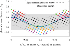
Figure 2. Illustration of the synthetic phason wave of figure 1 in an image with one direction of the physical space and one direction of the complementary space. The horizontal direction corresponds to the x-direction of the physical space (in which the phason wavevector  lies), and the vertical direction denotes the w1-direction in complementary space of the phason polarisation. Coloured squares again mark flipped particles, with the same colour code as in figure 1. The shaded area gives the projection of the envelope of the acceptance domain of the quasicrystal without phasonic distortion, the thin dotted curves describe the domain as modulated by the phasonic wave (overlaid as a bold dashed curve). The bold blue curve is the result of the phason reconstruction algorithm described in section 2.3.
Download figure:
Standard image High-resolution image2.3. Reconstruction of hyperspace embedding
In this section we discuss the analysis of phonons and phasons in a quasicrystal by reconstructing its embedding into hyperspace. In addition to the analysis of phonons, which can be straightforwardly carried out in physical space, this will give indications about the phasonic distortions underlying the observed flip patterns.
Basically, the reconstruction is achieved by reversing the projection procedure described in the previous section. For any two-dimensional particle configuration derived from a decagonal quasicrystal with known origin, one can construct an embedding into hyperspace as explained in the following. First, each particle i of the test pattern is embedded into five-dimensional space at the location  parametrised by its physical-space coordinates
  .
.
The particle i is then assigned to the hyperlattice site  closest to its position. In order to eliminate the trivial
  component from the embedding, we project the five-dimensional integer lattice onto a subspace orthogonal to
  . The hyperspace points that are assigned to a lattice point
  correspond to a four-dimensional Voronoi cell around that point. The residual parts of coordinates
  carry, separated into the physical and complementary directions, the information about phononic (
 ) and phasonic (
 ) displacements, respectively. In this way, we are able to reconstruct four-dimensional occupations from two-dimensional information, as long as deviations from an ideal embedded crystal are small compared to the extent of the acceptance domain, or rather the extension of the four-dimensional Voronoi cell.
In effect, we assign each physical particle to a point in hyperspace. The phononic offset is fully recovered, and all the residuals  indeed collapse to the origin if no phonons are present. The phasonic residuals
  fall into the acceptance domain in complementary space, and fill it densely in the infinite-system limit. Displays of the residual phasonic coordinates along
  and
and  are given as insets of figure 1 and the systems in section 3 with the central decagonal domain containing all particles which have not been flipped (black dots).
In the hyperspace picture, a phasonic flip corresponds to an assignment of a particle to an adjacent lattice site, so that its complementary-space coordinates lie outside the acceptance domain of the original lattice site (coloured squares in inset of figure 1). Conversely, the physical directions of the embedding contain the phononic part of particle motions between an idealised template and the analysed structure. This decoupling between phononic and phasonic movements effectively separates the two modes of hyperspace displacement. We exploit this to identify phasonic flips.
We now proceed to describe our analysis method for the system as a whole, to extract amplitudes of collective phononic and phasonic excitations. We apply the downhill simplex optimisation algorithm [38] to determine the amplitudes of a set of modes which have been chosen in advance. Our choice are plane waves with amplitudes and polarisations given by  and
and  for the phononic and phasonic part of the distortion space, respectively. In order to avoid mixing amplitude-type and phase-type variables, we use as orthogonal basis the harmonic functions
  ,
,  .
.
The reconstruction of a phononic displacement field by embedding it into the hyperspace is lossless. Therefore, we may extract the field directly by applying the downhill simplex optimisation to an energy functional that is proportional to the sum of phononic misfits (excluding jumped particles).
In contrast, the reconstruction of phason modes uses a more sophisticated energy functional: given the current parameter set, a trial system is constructed by the method described in section 2.2. Its particle placements are evaluated with penalties for false predictions. With the goal of an approximative recovery of thermal systems in mind, we design the energy functional to be a continuous function of the distortion amplitudes. Rather than a hard binary hit-or-miss criterion, we choose the error function, as a function of distance from the edge of the acceptance domain, to penalise badly-placed particles. The downhill simplex algorithm now minimises the difference in distribution of particles between the probed system and trial configurations. During the optimisation run, the sigmoid width of the error function is reduced, starting from a value of  , reduced step-wise by an overall factor of two.
The result of these two schemes is a quantitative interpretation of how the real-space distortions and phasonic jumps can be understood by deformations of the physical plane within its embedding into hyperspace.
2.4. Brownian dynamics simulations
We study thermally activated phononic and phasonic excitations in colloidal quasicrystals by employing Brownian dynamics simulations. In the simulations, we integrate the overdamped Langevin equation
with friction coefficient γ and position  of the particle in two dimensions. The random thermal force
  complies with
  and
and  where kB is the Boltzmann constant and T the temperature of the system. The internal force
  results from a pair potential V(r) such that
  with
with  ,
,  denotes the distance between two particles i and j.
The particles in our system interact through the Lennard-Jones–Gauss potential [33, 34]
with the energy unit  . For the parameters
  ,
,  and
and  , VLJG describes a double-well potential with two incommensurate length scales (see figure 3), favouring local decagonal symmetry and supporting quasicrystalline structures [33].

Figure 3. The Lennard-Jones–Gauss pair potential (blue curve) with its two length scales  and
and  . It is overlaid by the pair correlation function (histogram of pair distances, orange) of a decagonal quasicrystal, as it is stabilised in a Brownian dynamics simulation using the potential. Note there is a mismatch between the minima of the pair potential and the characteristic length scales in the quasicrystal, especially for the Lennard-Jones minimum.
Download figure:
Standard image High-resolution imageOur simulation quantities are dimensionless: energies are given relative to  , and temperatures T in terms of
  . The time unit is given by the Brownian time
  . We choose
  for a single Brownian dynamics time step. Furthermore, we apply a cut-off radius
  and subtract the cutoff force
  to ensure continuity. We determine the unit distance
  as the length scale of the pair potential such that—in accordance with the barostat used in references [33, 34]—a pressure-free system at T = 0 is achieved. Note there is a substantial detuning of the Lennard-Jones minimum relative to the pair distances of the actual system (figure 3), in contrast to the near-perfect match of the Gauss minimum.
We obtain initial positions of the particles from the projection method using a periodic approximant. The systems are heated up and held at a constant temperature for  , so that thermal equilibrium is reached. We remain well below the melting temperature
  from [34]. Prior to analysis, systems are instantaneously quenched: we continue the Brownian dynamics simulation at T = 0 for a duration of
  to allow the particles to find the equilibrium positions in their local environment, i.e. to freeze out phononic thermal noise.
3. Results and discussion
We now present the first applications of our analysis method. First, we determine the number of phasonic flips that result from a synthetic phason. Second, we analyse a synthetic phason in order to test our method. Third, we explore how thermally excited phasonic flips and phonon modes can be extracted from an intrinsic colloidal quasicrystal. Finally, we study the decay dynamics of synthetically excited phasons.
3.1. Phason amplitudes and numbers of phasonic flips
We first determine the number of phasonic flips which are introduced by a phasonic excitation with respect to the reference state. The phasonic excitation is constructed by choosing a set of mutually orthogonal harmonics with respect to the box size. To each individual mode  , a random amplitude vector
  and a random phase are assigned. We quantify the total magnitude of the excitation W by the sum of the absolute values of the amplitudes of the individual modes, i.e.
  .
.
Figure 4 (left) displays the phasonic flip fraction, i.e. the number of flipped particles divided by the total number of particles, as a function of the total amplitude W of the phasonic excitation. We find that the flip fraction increases linearly with the total amplitude and therefore with the amplitude of phasonic strain. Under the premise that all particle jumps in a given configuration are caused by phasonic excitations, this relationship could be used to estimate the total phasonic amplitude from the number of flips. Surprisingly, the number of wavevectors in the mode set seems to be insignificant, i.e. it is irrelevant if the total amplitude is contained in a single harmonic or in arbitrarily many modes.

Figure 4. Left: Fraction of flipped particles in systems with a single or multiple synthetic phasons dependent on the total amplitude W. The dotted line shows the slope of a linear relation. Right: Flip fractions after a Brownian dynamics annealing as a function of inverse temperature. The data scatter around an Arrhenius fit (green line).
Download figure:
Standard image High-resolution imageFigure 4 (right) displays the flip fraction found after annealing by using Brownian dynamics simulations of duration  as a function of the inverse temperature. The flip fraction exhibits Arrhenius behaviour
  with
with  and is compatible with a thermal activation of phasonic waves.
3.2. Recovery of known phasons from flip pattern
In this section we test the reliability of recovering a single, known phasonic excitation from a flip pattern that was constructed using the method described in section 2.2. An example of such a system is given in figure 1. We now apply the optimisation algorithm of section 2.3, restricted to the known phasonic wavevector. As can be seen in figure 2, the recovery result (blue bold line) agrees well with the original phason wave (black dashed line). The top panel of figure 5 displays where particles were flipped (black squares) due to the synthesised phason. In addition, we show where the best-fit reconstructed phason wave predicts the deletion (blue circle) and insertion (red) of particles. In  of the created and
  of the deleted particle positions, the fit agrees with the synthetic test system, hence the majority of flips has been correctly interpreted. False predictions usually occur if particles in hyperspace are close to the border of the acceptance domain (indicated by a lighter colour in the top pane of figure 5). Part of these discrepancies are due to the deliberate smoothening of the energy functional that we use for optimisation.

Figure 5. Applying the phason fit method to recover the flip configuration from the the synthetic phason shown in figures 1 and 2. Bottom: recovered phason wave where the w1-displacement is given by the colour code. Black squares are flipped particles. Top: magnification of the marked rectangle. Phasonic flips in the test pattern are denoted by black squares, with the jump vector attached to it. Particles disappearing or appearing due to the recovered phasonic field are indicated by blue and red circles, respectively. Point colours are lightened if embedded phasonic coordinates lie close to the border of the acceptance domain.
Download figure:
Standard image High-resolution imageThe quality of recovery of synthetic phasons depends on the wavelength of the phason. As figure 6 demonstrates, the recovery improves with the wavelength of the phasonic wave. The spatial resolution of a phason mode is limited by the typical distance between particles, making short-wavelength phasons less well-defined. Phasons with wavelengths  are discovered with good accuracy.

Figure 6. Recovery of a single-mode synthetic phason via our fit procedure depending on its wavelength λ. The recovered fraction of phason amplitude (ordinate) and mismatch in phase and polarisation (colour scale) are reasonable for long-wavelength modes, and decline when the wavelength gets closer to the inter-particle length scale  . The absolute value
  of the phason amplitude that we try to recover is encoded into point size, ranging
  . Its influence is minor, only accounting for a slightly increased variance in amplitude and polarisation recovery for low amplitudes.
Download figure:
Standard image High-resolution image3.3. Creation of excitations by annealing
We now explore what kind of excitations occur due to thermal fluctuations and how we can analyse them. We use excitation-free quasicrystals as starting configurations of Brownian dynamics simulations at constant temperature T. Noticeable numbers of phasonic flips start to occur above T = 0. 2 (compare with right-hand panel of figure 4). The vast majority of these flips persist when the system is quenched to T = 0 for analysis. These phasonic flips support, even at T = 0, a static phononic displacement field. Below T = 0.35, we find that the phonon field is typically dominated by a transversal (1, 0) mode aligned with the long dimension of the simulation box. Figure 7 illustrates this effect: after annealing for  at T = 0.300 the final configuration differs by 82 phasonic flips from the initial configuration. The flips enable a phononic strain field that does not level out at T = 0.

Figure 7. Top: quasicrystal in physical space, annealed by Brownian dynamics simulations at temperature T = 0.300. Phononic displacements are encoded into point sizes with the point area proportional to the displacement distance; flipped particles are represented by squares. Besides local strain fields around flips, an almost sinusoidal displacement profile has formed, corresponding to a transversal (u2-polarised) phonon. The inset denotes the positions in complementary space. Bottom: u2 displacement and the reconstructed phononic field obtained by optimising six modes.
Download figure:
Standard image High-resolution imageWe now use our optimisation procedure to extract the amplitudes of the six longest-wavelength modes ( ). For the system shown in figure 7, we find that the majority of strain lies within the transversal (1, 0) mode with amplitude
  , while the other modes vanish within fit accuracy (
 ). The best-fit results are consistent between successive runs of the optimisation with different random initial parameters. A system with a larger number of particles is shown in figure 8. In this case, a different approximant is used (see section 2.1), and the quasicrystal is rotated by 90 degrees with respect to the long dimension of the box. Again, a transversal phonon mode dominates the displacement field, but in this larger system, it is accompanied by additional long-wavelength harmonics.
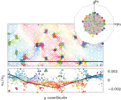
Figure 8. Top: quasicrystal annealed by Brownian dynamics, T = 0.300, larger system than in figure 7 and with a different approximant, which rotates the orientation by  (x and y directions swapped for depiction purposes; colour code stays identical to figure 1 with respect to the visible box orientation). A fit to the phononic displacements with the six longest-wavelength harmonic waves has been conducted. Bottom: the transversal phononic displacement u1. It is overlaid with the u1 component of the fit phonon field (bold line), evaluated along the line in the top image.
Download figure:
Standard image High-resolution imageNext, we want to interpret flips as manifestation of a continuous phasonic displacement field. Again, we consider the system of figure 7. In the optimisation procedure, we use the same modes as for the phonon fit, but with phasonic polarisations. In the bottom pane of figure 9, we display the best-fit phasonic displacement field within these modes. No mode clearly dominates the phason field. The total amplitude amounts to  , with the largest contribution coming from a (2, 0) mode with
  and elliptical polarisation. When we interpret the density of flips in the annealed system in the context of section 3.1, we expect the summed phason amplitude at about
  , which is in reasonable agreement with the value of W determined in this section by the optimisation method.

Figure 9. Phason recovery for a system annealed at T = 0.300, presentation identical to figure 5. Bottom: phasonic displacement field (intensity proportional to magnitude of displacement) as the result of the multi-mode fit process, flipped particles as black squares. Top: observations of Brownian dynamics flips (black) and those in the fit (red, blue).
Download figure:
Standard image High-resolution imageThe phason fit is less reliable than the phonon fit. For different initial parameters, the phason fit yields parameter sets which vary within a standard deviation of about  . Furthermore, the top pane of figure 9 demonstrates that the optimisation performs worse when predicting the phasonic flips in the Brownian dynamics simulations than for synthetic phasons. Overall,
  of the created and
  of the deleted particles agree between the annealed configuration and the recovered phasonic field. Note that wrong predictions are concentrated on particles close to the boundary of the acceptance domain (light coloured circles) while flips of particles well within the acceptance domain are usually described correctly (intense coloured circles).
The fraction of correctly characterised flips in principle could be increased by including phason modes with shorter wavelength into the optimisation process. On the other hand, with an increasing number of parameters, the deviations of the final parameters for different initialisations would further increase. Inherently, long-wavelength harmonics can only account for flip events that occur coherently though the whole system. Hence the optimisation systematically ignores strongly localised flip patterns, e.g. driven by thermal fluctuations. Nevertheless, with our choice of mode selection, we are able to extract the smooth part of the phasonic field, at the cost of ignoring localised effects.
In a continuum picture, phononic and phasonic strain fields are expected to be coupled [3]. In principle, one could conclude from this that a continuous phasonic strain field (evidenced by frozen-in phasonic flips) might give rise to the observed static phononic distortions. Our analysis does not reveal any strong correlation between the observed phonon modes and the dominant phasonic modes. However, as shown above, a large fraction of observed phasonic flips cannot be accounted for without shorter-wavelength phasons. In this limit, a continuum description of the quasicrystal might not be appropriate, such that the phonon/phason coupling is not observed on the atomic scale.
3.4. Dynamics of synthetic phasons during annealing
Phasonic strain usually is not relaxed at zero temperature: in order to flip a particle one has to cross an energy barrier. However, thermal fluctuations can in principle enable the system to overcome energy barriers and level out phasonic strain. Therefore, we study the relaxation of synthetic phasonic strain fields during Brownian dynamics annealing.
We start with a synthetic single-mode phason and track the relaxation of its amplitude over Brownian dynamics simulation time. Its amplitude may relax, and its phase and polarisation may drift with respect to the original phason. One test system exhibits a (1, 0) mode corresponding to a wavelength of  and a phasonic amplitude of
  . A second system has a (2, 3) mode, i.e. a shorter wavelength of
  and an amplitude of
  . The relaxation of both systems is studied at two temperatures, T = 0.2 and T = 0.3. We take periodic snapshots and fit a phasonic wave to each. The amplitude of the recovered phasons is shown in figure 10 as a function of time. As shown by the colour code, drifts of the phase and changes of the polarisation stay small during our simulation.

Figure 10. Systems with given synthetic phasonic waves are exposed to annealing by Brownian dynamics simulations. As a function of time, the particle configurations at different times are fitted to recover phason amplitude. The sum of a possible phase shift or change of polarisation with respect to the original phason is given by the colour code (identical to figure 6). Phasonic waves with very long wavelengths stay stable within the simulation time, whereas shorter-wavelength phasons tend to balance out. The higher the temperature, the faster the amplitude decays.
Download figure:
Standard image High-resolution image
For the temperatures considered, the magnitude of the (1, 0) mode shows no indications of relaxation in the presence of thermal noise. Some phase or polarisation misfit is determined from the beginning of the simulation, but it stays constant during the simulation. With its shorter wavelength, the (2, 3) mode behaves differently: initially, a fast, relaxation-like process reduces the amplitude. Then, the amplitude stabilises at a saturation level which is lower for higher temperatures. Our results may be rationalised considering the fact that, at the same amplitudes, the phasonic strain becomes more localised for shorter wavelengths, which might be conductive to relaxation. The saturation indicates that depending on the temperature there is a certain amount of phasonic stress that can prevail in the system. In other words, the phasonic stress associated with the saturation amplitudes is not large enough to initiate correlated phasonic flips that would be necessary to further relax the system.
4. Conclusions
We have examined phononic and phasonic excitations of two-dimensional decagonal quasicrystals. Our approach combines the synthesis of quasicrystalline patterns, analysis of physical-space location information, and interpretation of excitations in terms of harmonic modes. This can be applied to all quasicrystalline systems of which the ideal structure can be obtained by a projection or section from higher-dimensional space. We quantify spatially non-uniform deviations of the hyperspace embedding in terms of their phononic (stretching) and phasonic (buckling) fields.
The problem of reconstructing the distortion fields from the physical-space coordinates is underdetermined. Nevertheless, our method succeeds in recovering phononic and phasonic distortion fields, especially in the long-wavelength limit. Moreover, we apply this method to probe the excitations which develop in quasicrystals through annealing with Brownian dynamics simulations. Phononic fits, based on a low-harmonic Fourier ansatz, describe residual strains in thermal systems well. As for phasonic strains, however, the same modes are insufficient to explain all phasonic flips. Hence, for the colloidal system considered, high-frequency phasonic strains corresponding to localised thermal excitations must be assumed as well.
For synthetic phasonic waves, subject to prolonged thermalisation, amplitude recovery reveals either stability or decay as a function of time, depending on the gradient of phasonic strain and temperature. Relaxation of phasonic gradients has previously been observed in phason field reconstructions of metallic alloys [32]. We demonstrate that similar processes occur in intrinsic colloidal quasicrystals. In addition, we find a significant degree of temperature-dependent phasonic noise, which is not captured by long-wavelength harmonics.
We are confident that our method, in combination with the known tools for the detection of dislocations [14, 20, 35], is useful to analyse quasicrystals. Quasicrystals, even when free of dislocations, may contain residual deviations from the ideal structure. For example, a dislocation-free quasicrystal grown from a seed might be far from perfect due to built-in local phasonic rearrangements [8]. For another example, namely intrinsic colloidal quasicrystals obtained by Brownian dynamics simulations with perfect initial structures, we have shown in this article that phasonic excitations and as a consequence finite phononic displacement fields even occur at zero temperature. Using our method, we are able to detect and quantify this type of imperfections.
Acknowledgments
JH and SK acknowledge financial support by the Deutsche Forschungsgemeinschaft (DFG) as part of the Research Unit Geometry and Physics of Spatial Random Systems (grant Me1361/12). MS and MM were supported by the DFG within the Emmy Noether programme (Schm2657/2). We thank R A Solórzano Kraemer, M Klatt and S Ziegler for helpful discussions.