The induced higher derivative Lorentz-violating Chern–Simons term at finite temperature

Lorentz symmetry is one of the most tested symmetries of nature. Nevertheless, it is nowadays believed not to be an exact symmetry. In fact, it has been argued in [1] that tiny spontaneous breaking of Lorentz symmetry might arise in the context of string theory. Thus, if we add Lorentz-violating terms to the standard model, this new theory, namely the standard-model extension (SME) [2, 3], can be viewed as the low-energy limit of a physically relevant fundamental theory in which spontaneous Lorentz violation occurs. Many experiments and observations have been conducted to detect physical effects due to the Lorentz violation and some constraints on the Lorentz-violating terms were obtained, as we can see in [4].

The most studied part of the SME presents renormalizable operators of mass dimension d = 3 and d = 4, consequently, the coefficients contracted with these operators have mass dimension d = 1 or are dimensionless, respectively. This part of the SME is known as the minimal SME. However, in the SME there are operators with mass dimension d ⩾ 5, which are nonrenormalizable, contracted with coefficients of mass dimension d ⩽ −1. Although these operators are likely to be especially relevant in searches involving very high energies, providing new corrections, there are few studies on them.

Recently, some studies on higher derivative Lorentz-violating terms, described by the higher mass dimension operator (d ⩾ 5) have been made, such as [5–18]. In particular, the work [13] on operators of arbitrary mass dimension in the quantum electrodynamics (QED) extension have shown that the general form of the higher derivative terms in the photon sector is given by

$$\begin{equation} S_{(d)}=\int {{\rm d}^4x}\, \mathcal {K}^{\alpha _1 \alpha _2 \cdots \alpha _d}_{(d)} A_{\alpha _1}\partial _{\alpha _3}\cdots \partial _{\alpha _d} A_{\alpha _2}, \end{equation} \tag{ 1 }$$

where d is the dimension of the tensor operator and $\mathcal {K}^{\alpha _1 \alpha _2 \cdots \alpha _d}_{(d)}$ has mass dimension 4 − d.

On the one hand, for CPT-even terms, the first four indices of the coefficient $\mathcal {K}^{\alpha _1 \alpha _2 \cdots \alpha _d}_{(d)}$ have symmetries of the Riemann tensor, and there is total symmetry in the remaining d − 4 indices. On the other hand, for CPT-odd terms, the coefficient $\mathcal {K}^{\alpha _1 \alpha _2 \cdots \alpha _d}_{(d)}$ is antisymmetric in the first three indices and symmetric in the last d − 3.

In this work, we study the fermion sector of the QED extended by a CPT-odd term, governed by the coefficient b_μ, namely $b_\mu \bar{\psi }\gamma _5\gamma ^\mu \psi$. From the fermion sector of this minimal QED extension at zero temperature, we know that through radiative corrections we can generate the higher derivative Chern–Simons term,

$$\begin{equation} S_{(5)}=\int {{\rm d}^4x}\, \mathcal {K}^{\mu \nu \rho \alpha \beta }_{(5)} A_{\mu }\partial _{\rho } \partial _{\alpha }\partial _{\beta } A_{\nu }, \end{equation} \tag{ 2 }$$

with $\mathcal {K}^{\mu \nu \rho \alpha \beta }_{(5)}\propto \epsilon ^{\mu \nu \rho \sigma } b_\sigma g^{\alpha \beta }$, as can be seen by expanding the results in [3, 19] or directly in [21, 20]. Our goal here is to calculate the generation of the above term (2) using the method of derivative expansion [22–25] as a preparation for the finite temperature analysis, which has never been studied. To complement this, we also address the question of large gauge invariance of this higher derivative term as well as the conventional Chern–Simons term, both at finite temperature. For issues related to the Chern–Simons term, $\mathcal{L}_{(3)} =\mathcal {K}^{\mu \nu \rho }_{(3)} A_{\mu }\partial _{\rho } A_{\nu }$, see [26–33] and references therein.

It is interesting to mention that the term (2) arises when the Myers–Pospelov bosonic term [8] is radiatively induced from the fermion sector [20]. Therefore, effects of finite temperature on the higher derivative Chern–Simons term are somehow related to effects on the Myers–Pospelov term. Thus, studies of this nature deserve consideration in order to better characterize the higher derivative Lorentz-violating models.

This paper has the following structure. In section 2, we analyze the fermion sector of the Lorentz-violating QED with the coefficient b_μ, performing radiative corrections and using derivative expansion to induce the higher derivative Chern–Simons term at zero temperature. At the end of the section, we look for constraints on the coefficient of the induced term imposed by experimental and observational data. In section 3, we continue to look at the same theory as in the previous section, but now we are interested in the behavior of the term (2) at finite temperature. The issue of large gauge invariance is discussed in section 4. Finally, we present a summary in section 5.

As our aim is to study the generation of higher derivative CPT-odd terms (2), we consider the fermion sector of the Lorentz-violating QED, given by

$$\begin{equation} \mathcal {L}=\bar{\psi }({\rm i}/\!\!\! {\partial }-m-/\!\!\! {A}-\gamma _5/\!\!\! {b})\psi , \end{equation} \tag{ 3 }$$

where the first three terms are the usual ones, and the last and unusual term, which is governed by the coefficient b^μ, is the one responsible for the Lorentz and CPT violation.

In order to perform this task, we prefer to use the method of derivative expansion (for details see [34]), which is more suitable for calculating the sum integrals of the finite-temperature approach.

Then, from (3), the effective action S_eff is defined as

$$\begin{equation} Z = \int D \bar{\psi } D \psi {\rm e}^{{\rm i}\int {\rm d}^4 x \bar{\psi }({\rm i}/\!\!\! {\partial }-m-/\!\!\! {A}-\gamma _5/\!\!\! {b})\psi } = {\rm e}^{{\rm i} S_{\mathrm{eff}}}, \end{equation} \tag{ 4 }$$

in which

$$\begin{equation} S_{\mathrm{eff}}=-{\rm i}\mathop {\mathrm{Tr}}\nolimits \ln (/\!\!\! {p}-m- /\!\!\! {A}-\gamma _5 /\!\!\! {b}). \end{equation} \tag{ 5 }$$

Now, we can easily rewrite the effective action as $S_{\mathrm{eff}}=S^{(0)}_{\mathrm{eff}}+S^{(1)}_{\mathrm{eff}}$, where $S_\mathrm{eff}^{(0)}=-{\rm i} \mathop {\mathrm{Tr}}\nolimits \ln {(/\!\!\! {p}-m- \gamma _5 /\!\!\! {b})}$ and

$$\begin{equation} S^{(1)}_{\mathrm{eff}}={\rm i} \mathop {\mathrm{Tr}}\nolimits \sum _{n=1}^{\infty }\frac{1}{n}\bigg[\frac{1}{/\!\!\! {p}-m-\gamma _5/\!\!\! {b}} /\!\!\! {A}\bigg]^n . \end{equation} \tag{ 6 }$$

As the term $S^{(0)}_{\mathrm{eff}}$ does not depend on the gauge field, we must focus only on the term $S^{(1)}_{\mathrm{eff}}$. To generate the higher derivative Chern–Simons term it is necessary to have two contributions of the gauge field. Thus, we take n = 2 in the expression (6) and use the following expansion for the fermionic propagator,

$$\begin{equation} \fl \frac{1}{/\!\!\! {p}-m-\gamma _5/\!\!\! {b}} = \frac{1}{/\!\!\! {p}-m}+\frac{1}{/\!\!\! {p}-m}\gamma _5/\!\!\! {b}\frac{1}{/\!\!\! {p}-m} +\frac{1}{/\!\!\! {p}-m}\gamma _5/\!\!\! {b}\frac{1}{/\!\!\! {p}-m}\gamma _5/\!\!\! {b}\frac{1}{/\!\!\! {p}-m}+\cdots , \end{equation} \tag{ 7 }$$

to single out contributions of first order in b_μ. It is worth emphasizing that the higher derivative Chern–Simons term (and the Myers–Pospelov term) is also induced when we consider contributions of third order in b_μ, as has been shown in [20]. Following on from the derivative expansion approach [22–25, 34], we find

$$\begin{equation} \fl S_{b}^{(1,2)}=\frac{{\rm i}}{2} \mathop {\mathrm{Tr}}\nolimits [S(p)\gamma ^\mu S(p-k)\gamma _5 /\!\!\! {b}S(p-k)\gamma ^\nu +S(p)\gamma _5 /\!\!\! {b}S(p)\gamma ^\mu S(p-k)\gamma ^\nu ]A_\mu A_\nu , \end{equation} \tag{ 8 }$$

where S(p) = (/p − m)⁻¹. Finally, expanding the propagator up to third order in k_μ,

$$\begin{equation} \fl S(p-k)= S(p)+S(p)/\!\!\! {k}S(p)+S(p)/\!\!\! {k}S(p)/\!\!\! {k}S(p)+S(p)/\!\!\! {k}S(p)/\!\!\! {k}S(p)/\!\!\! {k}S(p)+\cdots , \end{equation} \tag{ 9 }$$

we obtain

$$\begin{equation} S_{(5)}=\frac{{\rm i}}{2}\int {\frac{{\rm d}^4k}{(2 \pi )^4}\Pi ^{\mu \nu }_{(5)}\, A_\mu (k) A_\nu (-k)}, \end{equation} \tag{ 10 }$$

with

$$\begin{eqnarray} &&\fl \Pi ^{\mu \nu }_{(5)} =\int \frac{{\rm d}^4 p}{(2\pi )^4} \mathop {\mathrm{tr}}\nolimits [S(p)\gamma ^\mu S(p)\gamma _5 /\!\!\! {b}S(p)/\!\!\! {k} S(p)/\!\!\! {k}S(p)/\!\!\! {k} S(p)\gamma ^\nu \nonumber \\ &&+\, S(p)\gamma ^\mu S(p)/\!\!\! {k} S(p)\gamma _5 /\!\!\! {b}S(p)/\!\!\! {k} S(p)/\!\!\! {k} S(p)\gamma ^\nu \nonumber \\ &&+\, S(p)\gamma ^\mu S(p)/\!\!\! {k} S(p)/\!\!\! {k} S(p)\gamma _5 /\!\!\! {b}S(p)/\!\!\! {k} S(p)\gamma ^\nu \nonumber \\ &&+\, S(p)\gamma ^\mu S(p)/\!\!\! {k} S(p)/\!\!\! {k} S(p)/\!\!\! {k} S(p)\gamma _5 /\!\!\! {b}S(p)\gamma ^\nu \nonumber \\ &&+\, S(p)\gamma _5 /\!\!\! {b}S(p)\gamma ^\mu S(p)/\!\!\! {k} S(p)/\!\!\! {k} S(p)/\!\!\! {k} S(p)\gamma ^\nu ], \end{eqnarray} \tag{ 11 }$$

where we have calculated the trace over the coordinate and momentum spaces and considered cubic terms of k_μ.

Before evaluating the integrals in (48), we first calculate the trace over the Dirac matrices, so that we have

$$\begin{eqnarray} \fl \Pi ^{\mu \nu }_{(5)}&=& 4{\rm i} \epsilon ^{\mu \nu \sigma \rho } b_\sigma k_\rho k^2\int { \frac{{\rm d}^4 p}{(2\pi )^4}}\frac{1}{(p^2-m^2)^3} - 16{\rm i} \epsilon ^{\mu \nu \sigma \rho } b_\sigma k_\rho k^\alpha k^\beta \int { \frac{{\rm d}^4 p}{(2\pi )^4}}\frac{p_\alpha p_\beta }{(p^2-m^2)^4}\nonumber \\ \ms \fl &&+\, 24{\rm i} m^2 \epsilon ^{\mu \nu \sigma \rho } b_\sigma k_\rho k^2 \int { \frac{{\rm d}^4 p}{(2\pi )^4}}\frac{1}{(p^2-m^2)^4} + 24{\rm i} \epsilon ^{\mu \nu \rho \alpha } k_\rho b^\beta k^2 \int { \frac{{\rm d}^4 p}{(2\pi )^4}}\frac{p_\alpha p_\beta }{(p^2-m^2)^4}\nonumber \\ \ms \fl &&+\, 32{\rm i} \epsilon ^{\mu \nu \rho \alpha }k_\rho (b\cdot k)k^\beta \int { \frac{{\rm d}^4 p}{(2\pi )^4}}\frac{p_\alpha p_\beta }{(p^2-m^2)^4} \nonumber\\ \fl &&-\, 128{\rm i} \epsilon ^{\mu \nu \sigma \rho } b_\sigma k_\rho k^\alpha k^\beta \int { \frac{{\rm d}^4 p}{(2\pi )^4}}\frac{p_\alpha p_\beta }{(p^2-m^2)^5}\nonumber\\ \fl &&-\, 128{\rm i} \epsilon ^{\mu \nu \rho \alpha } k_\rho b^\beta k^\delta k^\gamma \int { \frac{{\rm d}^4 p}{(2\pi )^4}}\frac{p_\alpha p_\beta p_\delta p_\gamma }{(p^2-m^2)^5}. \end{eqnarray} \tag{ 12 }$$

Now, by analyzing the above integrals we observe that, after a simple power counting, we do not need to use regularization schemes because all integrals are convergent. Therefore, we can solve (12) directly by using well-known solutions in which the higher derivative Chern–Simons term is given by

$$\begin{equation} \Pi ^{\mu \nu }_{(5)}=-\frac{\epsilon ^{\mu \nu \sigma \rho } b_\sigma k_\rho k^2}{12 m^2 \pi ^2}, \end{equation} \tag{ 13 }$$

or through the following Lagrangian as

$$\begin{equation} \mathcal {L}_{(5)}=\frac{e^2}{24 m^2 \pi ^2} \epsilon ^{\mu \nu \rho \sigma } b_\sigma A_\mu \partial _\rho \Box A_\nu , \end{equation} \tag{ 14 }$$

with $\mathcal {K}^{\mu \nu \rho \alpha \beta }_{(5)}= \frac{e^2}{24 m^2 \pi ^2}\epsilon ^{\mu \nu \sigma \rho } b_\sigma g^{\alpha \beta }$, where we have reinstalled the electron charge.

The higher derivative Chern–Simons term (14) is also induced through radiative corrections from another CPT-odd term of the SME, namely governed by the coefficient g^μνρ, when g^μνρ is totally antisymmetric [15].

Numerical estimates for the coefficient b_μ of the higher derivative Chern–Simons term can be obtained from bounds on the coefficient $\mathcal {K}^{\mu \nu \rho \alpha \beta }_{(5)}$ of the photon sector (see [4], table XIX). From observational data related to the cosmic microwave background polarization, we can estimate b ∼ 10⁻²⁴. Moreover, from systems related to the astrophysical birefringence, we estimate that the coefficient is ∼10⁻³⁶. In these estimates we have considered m as being the electron mass, m ≃ 0.5 × 10⁻³ GeV, and e ≃ 10⁻¹ as the electron charge. In this way, we observe that we have found tiny values for the coefficient b_μ compatible with maximal sensitivities for the electron sector (table II of [4]).

In this section, we are interested in the finite temperature behavior of the higher derivative term (13). For this, we take the equation (12) and change it from Minkowski space to Euclidean space. We would like to emphasize here that the method of derivative expansion used above, in general, is rather delicate at finite temperature, due to the fact that the limits k₀ → 0 and $\vec{k}\rightarrow 0$ do not commute, arising from the non-analyticity of thermal amplitudes [35]. In the expression (12) we have considered the limits k₀ → 0 and $\vec{k}\rightarrow 0$. Then, by performing the procedure p₀ → ip₀ (g^μν → −δ^μν), d⁴p → id⁴p_E, and $p^2\rightarrow -p_0^2-\vec{p}^{\,2} = -p^2_E$, we obtain

$$\begin{eqnarray} \fl \Pi ^{\mu \nu }_{(5)}&=& {-}4 \epsilon ^{\mu \nu \sigma \rho } b^\sigma _E k^\rho _E k^2_E \int {\frac{{\rm d}^4 p_E}{(2 \pi )^4}}\frac{1}{(p^2_E + m^2)^3} + 16 \epsilon ^{\mu \nu \sigma \rho } b^\sigma _E k^\rho _E k^\alpha _E k^\beta _E \int {\frac{{\rm d}^4 p_E}{(2 \pi )^4}}\frac{p^\alpha _E p^\beta _E}{(p^2_E + m^2)^4}\nonumber \\ \ms \fl &&+\, 24 m^2 \epsilon ^{\mu \nu \sigma \rho } b^\sigma _E k^\rho _E k^2_E \int {\frac{{\rm d}^4 p_E}{(2 \pi )^4}}\frac{1}{(p^2_E + m^2)^4} - 24 \epsilon ^{\mu \nu \rho \alpha } k^\rho _E b^\beta _E k^2_E \int {\frac{{\rm d}^4 p_E}{(2 \pi )^4}}\frac{p^\alpha _E p^\beta _E}{(p^2_E + m^2)^4}\nonumber \\ \ms \fl &&-\, 32 \epsilon ^{\mu \nu \rho \alpha }k^\rho _E (b_E\cdot k_E)k^\beta _E \int {\frac{{\rm d}^4 p_E}{(2 \pi )^4}}\frac{p^\alpha _E p^\beta _E}{(p^2_E + m^2)^4} \nonumber\\ \fl &&-\, 128 \epsilon ^{\mu \nu \sigma \rho } b^\sigma _E k^\rho _E k^\alpha _E k^\beta _E \int {\frac{{\rm d}^4 p_E}{(2 \pi )^4}}\frac{p^\alpha _E p^\beta _E}{(p^2_E + m^2)^5} \nonumber \\ \fl &&+\, 128 \epsilon ^{\mu \nu \rho \alpha } k^\rho _E b^\beta _E k^\delta _E k^\gamma _E \int {\frac{{\rm d}^4 p_E}{(2 \pi )^4}}\frac{p^\alpha _E p^\beta _E p^\delta _E p^\gamma _E}{(p^2_E + m^2)^5}. \end{eqnarray} \tag{ 15 }$$

In order to effectively tackle the issue of the finite temperature behavior of the above expression, we separate the space and time components of the 4-momentum $p^\sigma _E=(p_0,\vec{p})$ as $p^\sigma _E\rightarrow \hat{p}^\sigma +p_0\delta ^{\sigma 0}$, so that $\hat{p}^\sigma =(0,\vec{p})$. Also, due to the symmetry of the integral under spatial rotations, it is possible to use the substitutions

$$\begin{equation} \hat{p}^\alpha \hat{p}^\beta \rightarrow \frac{\hat{p}^2}{3}(\delta ^{\alpha \beta }-\delta ^{\alpha 0} \delta ^{\beta 0}) \end{equation} \tag{ 16 }$$

and

$$\begin{eqnarray} &&\fl \hat{p}^\alpha \hat{p}^\beta \hat{p}^\delta \hat{p}^\gamma \rightarrow \frac{\hat{p}^4}{15}[(\delta ^{\alpha \beta }-\delta ^{\alpha 0}\delta ^{\beta 0})(\delta ^{\delta \gamma }-\delta ^{\delta 0}\delta ^{\gamma 0})+(\delta ^{\alpha \delta }-\delta ^{\alpha 0}\delta ^{\delta 0})(\delta ^{\beta \gamma }-\delta ^{\beta 0}\delta ^{\gamma 0})\nonumber \\ &&+(\delta ^{\alpha \gamma }-\delta ^{\alpha 0}\delta ^{\gamma 0})(\delta ^{\beta \delta }-\delta ^{\beta 0}\delta ^{\delta 0})]. \end{eqnarray} \tag{ 17 }$$

After applying these changes to equation (15), we find seven different tensorial structures. The first two structures, $\epsilon ^{\mu \nu \sigma \rho } k^{\sigma }_E k^{\rho }_E b^0_E k^0_E$ and $\epsilon ^{\mu \nu \sigma \rho } k^{\sigma }_E k^{\rho }_E (b_E \cdot k_E)$, obviously vanish by antisymmetry of ^μνσρ. In addition, the third contribution, $\epsilon ^{\mu \nu 0 \sigma } k^{0}_E k^{\sigma }_E (b_E \cdot k_E)$, goes to zero after the integration in the space components of $p_E^\alpha$. Therefore, we are left with four different structures to analyze, namely $\epsilon ^{\mu \nu \sigma \rho } b^{\sigma }_E k^{\rho }_E k^2_E$, $\epsilon ^{\mu \nu 0 \rho } b^{0}_E k^{\rho }_E k^2_E$, $\epsilon ^{\mu \nu \sigma \rho } b^{\sigma }_E k^{\rho }_E (k^0_E)^2$ and $\epsilon ^{\mu \nu 0 \rho } b^{0}_E k^{\rho }_E (k^0_E)^2$. Thus, we have $\Pi ^{\mu \nu }_{(5)}=\Pi ^{\mu \nu }_{(a)}+\Pi ^{\mu \nu }_{(b)}+\Pi ^{\mu \nu }_{(c)}+\Pi ^{\mu \nu }_{(c)}$, with the following expressions for these four tensorial structures:

$$\begin{eqnarray} &&\fl \Pi ^{\mu \nu }_{(a)}= -4 \epsilon ^{\mu \nu \sigma \rho } b^{\sigma }_E k^{\rho }_E k^2_E \int \frac{{\rm d}p_0}{2 \pi }\bigg[ \frac{32}{15}I_1(p_0,m)+\frac{32 m^2}{3} I_2(p_0,m)-\frac{10}{3} I_4(p_0,m) \nonumber \\ &&- 6 m^2 I_5(p_0,m)+ I_6(p_0,m)\bigg ], \end{eqnarray} \tag{ 18 }$$

$$\begin{eqnarray} &&\fl \Pi ^{\mu \nu }_{(b)}= 8 \epsilon ^{\mu \nu 0 \rho } b^{0}_E k^{\rho }_E k^2_E \int \frac{{\rm d}p_0}{2 \pi } \bigg[ \frac{16}{15}I_1(p_0,m)-\frac{16}{3}p_0^2 I_2(p_0,m) - I_4(p_0,m) + 3p_0^2 I_5(p_0,m)\bigg], \nonumber \\ \end{eqnarray} \tag{ 19 }$$

$$\begin{eqnarray} &&\fl \Pi ^{\mu \nu }_{(c)}= -16 \epsilon ^{\mu \nu \sigma \rho } b^{\sigma }_E k^{\rho }_E (k^0_E)^2\int \frac{{\rm d}p_0}{2 \pi }\bigg[ -\frac{8}{15}I_1(p_0,m)+\frac{8}{3}(p_0^2-m^2)I_2(p_0,m) \nonumber \\ &&+8 p_0^2 m^2 I_3(p_0,m) + \frac{1}{3} I_4(p_0,m)-p_0^2I_5(p_0,m)\bigg], \end{eqnarray} \tag{ 20 }$$

$$\begin{equation} \fl \Pi ^{\mu \nu }_{(d)}= -128\epsilon ^{\mu \nu 0 \rho } b^{0}_E k^{\rho }_E (k^0_E)^2 \int \frac{{\rm d}p_0}{2 \pi }\bigg[ \frac{1}{5}I_1(p_0,m)-2 p_0^2 I_2(p_0,m)+p_0^4 I_3(p_0,m)\bigg], \end{equation} \tag{ 21 }$$

where the integrals I_{1, 2, 3, 4, 5, 6}(p₀, m) are given by

$$\begin{equation} I_{1,2,3}(p_0,m)= \int \frac{{\rm d}^3p_E}{(2 \pi )^3}\frac{\alpha _{1,2,3}}{(\vec{p}^{\,2}+p_0^2+m^2)^5}, \end{equation} \tag{ 22 }$$

$$\begin{equation} I_{4,5}(p_0,m)= \int \frac{{\rm d}^3p_E}{(2 \pi )^3}\frac{\alpha _{4,5}}{(\vec{p}^{\,2}+p_0^2+m^2)^4}, \end{equation} \tag{ 23 }$$

$$\begin{equation} I_6(p_0,m)= \int \frac{{\rm d}^3p_E}{(2 \pi )^3}\frac{1}{(\vec{p}^{\,2}+p_0^2+m^2)^3}, \end{equation} \tag{ 24 }$$

with $\alpha _1=\vec{p}^4,\alpha _2=\alpha _4=\vec{p}^{\,2}$ and α₃ = α₅ = 1.

Now, we calculate the integrals over the space components $\vec{p}$. This can be done without using regularization schemes, because all the integrals are convergent. Then, we find

$$\begin{eqnarray} &&\fl \Pi ^{\mu \nu }_{(a)}=\frac{m^2}{ 8\pi }\epsilon ^{\mu \nu \sigma \rho } b^{\sigma }_E k^{\rho }_E k^2_E \bigg[\int \frac{{\rm d}p_0}{2 \pi }(p_0^2+m^2)^{-\frac{5}{2}}-\frac{2}{3m^2}\int \frac{{\rm d}p_0}{2 \pi }(p_0^2+m^2)^{-\frac{3}{2}}\bigg], \nonumber \\ &&+\frac{1}{12\pi }\epsilon ^{\mu \nu \sigma \rho } b^{\sigma }_E k^{\rho }_E k^2_E \int \frac{{\rm d}p_0}{2 \pi }(p_0^2+m^2)^{-\frac{3}{2}} \end{eqnarray} \tag{ 25 }$$

$$\begin{equation} \fl \Pi ^{\mu \nu }_{(b)} = -\frac{m^2}{8 \pi }\epsilon ^{\mu \nu 0 \rho } b^{0}_E k^{\rho }_E k^2_E \bigg[\int \frac{{\rm d}p_0}{2 \pi }(p_0^2+m^2)^{-\frac{5}{2}}-\frac{2}{3m^2}\int \frac{{\rm d}p_0}{2 \pi }(p_0^2+m^2)^{-\frac{3}{2}}\bigg], \end{equation} \tag{ 26 }$$

$$\begin{equation} \fl \Pi ^{\mu \nu }_{(c)}= \frac{ m^2}{ \pi }\epsilon ^{\mu \nu \sigma \rho } b^{\sigma }_E k^{\rho }_E (k^0_E)^2\bigg[\frac{5 m^2}{4} \int \frac{{\rm d}p_0}{2 \pi }(p_0^2+m^2)^{-\frac{7}{2}}-\int \frac{{\rm d}p_0}{2 \pi }(p_0^2+m^2)^{-\frac{5}{2}}\bigg], \end{equation} \tag{ 27 }$$

$$\begin{equation} \fl \Pi ^{\mu \nu }_{(d)}= -\frac{m^2}{\pi }\epsilon ^{\mu \nu 0 \rho } b^{0}_E k^{\rho }_E (k^0_E)^2 \bigg[\frac{5 m^2}{4} \int \frac{{\rm d}p_0}{2 \pi }(p_0^2+m^2)^{-\frac{7}{2}}-\int \frac{{\rm d}p_0}{2 \pi }(p_0^2+m^2)^{-\frac{5}{2}}\bigg]. \end{equation} \tag{ 28 }$$

Note that $\Pi ^{\mu \nu }_{(b)}$ and $\Pi ^{\mu \nu }_{(d)}$ cancel the corresponding time components $b_E^0$ of $\Pi ^{\mu \nu }_{(a)}$ and $\Pi ^{\mu \nu }_{(c)}$, respectively. Therefore, by summing all expressions, we obtain

$$\begin{eqnarray} \fl \Pi ^{\mu \nu }_{(5)} &=& -\frac{1}{m^2}\epsilon ^{\mu \nu \sigma \rho } b^{\sigma }_E k^{\rho }_E k^2_E B(m) - \frac{1}{m^2}\epsilon ^{\mu \nu i \rho } b^{i}_E k^{\rho }_E k^2_E C_1(m)- \frac{1}{m^2}\epsilon ^{\mu \nu i \rho } b^{i}_E k^{\rho }_E (k^0_E)^2 C_2(m), \end{eqnarray} \tag{ 29 }$$

where

$$\begin{equation} B(m) = -\frac{m^2}{12 \pi } \int \frac{{\rm d}p_0}{2 \pi }(p_0^2+m^2)^{-\frac{3}{2}}, \end{equation} \tag{ 30a }$$

$$\begin{equation} C_1(m) = \frac{m^2}{12\pi }\int \frac{{\rm d}p_0}{2 \pi }(p_0^2+m^2)^{-\frac{3}{2}} - \frac{m^4}{8 \pi }\int \frac{{\rm d}p_0}{2 \pi }(p_0^2+m^2)^{-\frac{5}{2}}, \end{equation} \tag{ 30b }$$

$$\begin{equation} C_2(m) = \frac{m^4}{\pi }\int \frac{{\rm d}p_0}{2 \pi }(p_0^2+m^2)^{-\frac{5}{2}} - \frac{5 m^6}{4 \pi } \int \frac{{\rm d}p_0}{2 \pi }(p_0^2+m^2)^{-\frac{7}{2}}, \end{equation} \tag{ 30c }$$

with i = 1, 2, 3.

The finite temperature behavior of the above terms can be obtained by using the Matsubara formalism. For this, we write $p_0=(n +1/2) \frac{2\pi }{\beta }$, which are the Matsubara frequencies, and change the integral over p₀ into a sum, $\frac{1}{2\pi }\int {{\rm d}p_0}\rightarrow \frac{1}{\beta }\sum _n$, where T = β⁻¹ is the temperature of the system. Assuming that $\xi =\frac{\beta m}{2 \pi }$, we can write B(m) → B(ξ), C₁(m) → C₁(ξ), and C₂(m) → C₂(ξ), so that

$$\begin{equation} \fl B(\xi ) = -\frac{\xi ^2}{24 \pi ^2}\sum _n{[(n+1/2)^2+\xi ^2]^{-3/2}}, \end{equation} \tag{ 31a }$$

$$\begin{equation} \fl C_1(\xi ) = \frac{\xi ^2}{24\pi ^2}\sum _n{[(n+1/2)^2+\xi ^2]^{-3/2}} - \frac{\xi ^4}{16\pi ^2} \sum _n{[(n+1/2)^2+\xi ^2]^{-5/2}} \end{equation} \tag{ 31b }$$

$$\begin{equation} \fl C_2(\xi ) = \frac{\xi ^4}{2 \pi ^2} \sum _n{[(n+1/2)^2+\xi ^2]^{-5/2}} - \frac{5 \xi ^6}{8\pi ^2}\sum _n{[(n+1/2)^2+\xi ^2]^{-7/2}}. \end{equation} \tag{ 31c }$$

As the above summations are all convergent, they can be easily evaluated numerically. Nevertheless, the asymptotic limits, zero and high temperatures, are not easy to obtain. One way to do this is to convert the sums into integrals, by using the expression [36]

$$\begin{equation} \sum \limits _{n}[(n+b)^2+a^2]^{-\lambda }=\frac{\sqrt{\pi }\Gamma (\lambda - 1/2)}{\Gamma (\lambda )(a^2)^{\lambda -1/2}}+ 4\sin (\pi \lambda ) f_\lambda (a,b), \end{equation} \tag{ 32 }$$

where

$$\begin{equation} f_\lambda (a,b)= \int \nolimits _{|a|}^{\infty } \frac{{\rm d}z}{(z^2-a^2)^\lambda } Re \bigg( \frac{1}{{\rm e}^{2\pi (z+{\rm i}b)}-1} \bigg), \end{equation} \tag{ 33 }$$

which is valid for Re λ < 1, aside from the poles at λ = 1/2, −1/2, −3/2, .... However, by analyzing the equations (31a)–(31c), we have the values λ = 3/2, λ = 5/2 and λ = 7/2, i.e. they are all out of range of validity. Luckily, we can use a recurrence relation, given by

$$\begin{equation} \fl f_{\lambda -1}(a,b)=-\frac{1}{2a^2}\frac{2\lambda -5}{\lambda -2}f_{\lambda -2}(a,b)-\frac{1}{4a^2}\frac{1}{(\lambda -3)(\lambda -2)}\frac{\partial ^2}{\partial b^2}f_{\lambda -3}(a,b), \end{equation} \tag{ 34 }$$

in order to decrease these values of λ. In this way, for λ = 3/2 we must use the recurrence relation once, for λ = 5/2 twice, and for λ = 7/2 thrice. We must also write λ = 3/2 → D/2, λ = 5/2 → D/2 + 1, and λ = 7/2 → D/2 + 2, to avoid the poles λ = 1/2, −1/2 in the first term of the solution (32), so that the expressions (31) become

$$\begin{equation} \fl B(\xi ) = -\frac{m^{3-D}}{24\pi ^2}\xi ^{D-1}\sum _n{[(n+1/2)^2+\xi ^2]^{-\frac{D}{2}}}, \end{equation} \tag{ 35a }$$

$$\begin{eqnarray} &&\fl C_1(\xi ) = \frac{m^{3-D}}{24\pi ^2}\xi ^{D-1}\sum _n{[(n+1/2)^2+\xi ^2]^{-\frac{D}{2}}} - \frac{m^{3-D}}{16\pi ^2}\xi ^{D+1}\sum _n{[(n+1/2)^2+\xi ^2]^{-\frac{D}{2}-1}}, \nonumber \\ \end{eqnarray} \tag{ 35b }$$

$$\begin{eqnarray} &&\fl C_2(\xi ) = \frac{m^{3-D}}{2 \pi ^2}\xi ^{D+1}\sum _n{[(n+1/2)^2+\xi ^2]^{-\frac{D}{2}-1}} - \frac{5m^{3-D}}{8\pi ^2}\xi ^{D+3}\sum _n{[(n+1/2)^2+\xi ^2]^{-\frac{D}{2}-2}}. \nonumber \\ \end{eqnarray} \tag{ 35c }$$

Then, by using the recurrence relation (34) and considering the sum (32), after we take the limit D → 3, we obtain

$$\begin{equation} \fl \Pi ^{\mu \nu }_{(5)} = \frac{1}{m^2}\epsilon ^{\mu \nu \sigma \rho } b_{\sigma } k_{\rho } k^2 B(\xi ) + \frac{1}{m^2} \epsilon ^{\mu \nu i \rho } b_{i} k_{\rho } k^2 C_1(\xi ) +\frac{1}{m^2}\epsilon ^{\mu \nu i \rho } b_{i} k_{\rho } k_0^2 C_2(\xi ), \end{equation} \tag{ 36 }$$

with

$$\begin{equation} B(\xi ) = \frac{1}{6}\int \nolimits _{|\xi |}^{\infty }{\rm d}z \sqrt{z^2-\xi ^2}\tanh (\pi z)\mathrm{sech}^2(\pi z)-\frac{1}{12 \pi ^2}, \end{equation} \tag{ 37a }$$

$$\begin{equation} C_1(\xi ) =\frac{\xi ^2}{12}\int \nolimits _{|\xi |}^{\infty }{\rm d}z\frac{ \tanh (\pi z)\mathrm{sech}^2(\pi z)}{ \sqrt{z^2-\xi ^2}}, \end{equation} \tag{ 37b }$$

$$\begin{equation} C_2(\xi ) = \frac{\pi ^2 \xi ^2}{6}\int \nolimits _{|\xi |}^{\infty }{\rm d}z\sqrt{z^2-\xi ^2}\mathrm{sech}^5(\pi z)[\sinh (3\pi z)-11\sinh (\pi z)], \end{equation} \tag{ 37c }$$

where we have returned to the Minkowski space.

By analyzing the above equations we observe that when T → 0 (ξ → ∞) all the integrals vanish, so that $\Pi ^{\mu \nu }_{(5)}$ goes to $-\frac{1}{12 \pi ^2 m^2}\epsilon ^{\mu \nu \sigma \rho } b_{\sigma } k_{\rho } k^2$. This is in fact the result of the zero temperature, obtained previously in (13). On the other hand, when T → ∞ (ξ → 0) the expression (37a) goes to zero, as well as the expressions (37b) and (37c). This happens mainly because all the summations in (31) are strongly suppressed by the temperature, thus suggesting that in general the operators of mass dimension d ⩾ 5 vanish in the limit of high temperature.

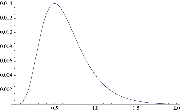
The plot of the functions B(ξ), C₁(ξ), and C₂(ξ), which can be numerically calculated from either expressions (31) or (37), are presented in figures 1–3. It is interesting to note here that these functions are the same as those obtained in the context of the coefficient g^μνρ [16]. This is because under a certain fermion field redefinition [2, 37] the totally antisymmetric component of g^μνρ is completely absorbed into coefficient b^μ.

Zoom In Zoom Out Reset image size

Zoom In Zoom Out Reset image size

Zoom In Zoom Out Reset image size

Let us now briefly discuss the question of large gauge invariance at finite temperature, in the context of Lorentz- and CPT-violating QED. This issue has been extensively studied in three-dimensional Chern–Simons theories [38–45]. In our case, we want to examine the invariance of the higher derivative Chern–Simons term (2) under large gauge transformation, as well as the four-dimensional Chern–Simons term, namely,

$$\begin{equation} S_{(3)}=\int {{\rm d}^4x}\, \mathcal {K}^{\mu \nu \rho }_{(3)} A_{\mu }\partial _{\rho } A_{\nu }, \end{equation} \tag{ 38 }$$

with $\mathcal {K}^{\mu \nu \rho }_{(3)}\propto \epsilon ^{\mu \nu \rho \sigma } b_\sigma$, where both are dynamically generated by the effective action (5). It would be interesting to consider the other terms with operators of mass dimension d = 7, 9, ...; however, this is a challenging task. In fact, in the literature we find only models with Lorentz-violating operators of mass dimension d = 5 for CPT-odd terms. In particular, we can argue that, as $\mathcal{K}_{(d)}\sim M_{{\rm Pl}}^{4-d}$, these operators with d ⩾ 7 are highly suppressed by the Planck mass M_Pl and are therefore even more negligible.

To perform this investigation, we continue to use the method of derivative expansion, in a particular gauge field background, however, where we have a vanishing electric field and a time-independent magnetic field, as follows

$$\begin{equation} A_0=A_0(t), \hspace{14.22636pt} A_i=A_i(x,y,z). \end{equation} \tag{ 39 }$$

It is worth mentioning that this specific choice of gauge background is consistent with the static limit, as shown in [44], although it is not a static background. The point here is that in this static limit we can avoid the non-analyticity of thermal amplitudes, which can appear when the effective action is expanded in powers of derivatives. Furthermore, in this background (39) we believe that the effective action can be calculated exactly.

Finally, by considering the appropriate gauge transformation [41, 42],

$$\begin{equation} A_\mu \rightarrow A_\mu + \partial _\mu \Omega , \hspace{14.22636pt} \Omega (t)=\bigg(-\int _0^t+\frac{t}{\beta }\int _0^\beta \bigg){\rm d}t^{\prime } A_0(t^{\prime }), \end{equation} \tag{ 40 }$$

we obtain

$$\begin{equation} A_0 \rightarrow \frac{a_0}{\beta }= \frac{1}{\beta }\int _0^\beta {\rm d}t\, A_0(t), \hspace{14.22636pt} A_i \rightarrow A_i(x,y,z), \end{equation} \tag{ 41 }$$

so that under large gauge transformation,

$$\begin{equation} a_0 \rightarrow a_0 + 2\pi n, \end{equation} \tag{ 42 }$$

where n is an integer. Then, by taking into account these constraints, we can rewrite the effective action (5) in the Euclidean space as

$$\begin{equation} S_{\mathrm{eff}}=-\sum _n\mathop {\mathrm{Tr}}\nolimits \ln (\vec{/\!\!\! {p}}+\tilde{\omega }_n\gamma ^0+m-\vec{/\!\!\! {A}}-\gamma _5 /\!\!\! {b}_E), \end{equation} \tag{ 43 }$$

in which we have introduced the definitions $\vec{/\!\!\! {p}}=p^i\gamma ^i$, /b_E = b⁰γ⁰ + bⁱγⁱ, and

$$\begin{equation} \tilde{\omega }_n=\omega _n-\frac{a_0}{\beta }=(n +1/2) \frac{2\pi }{\beta }-\frac{a_0}{\beta }. \end{equation} \tag{ 44 }$$

Now, following the procedure performed in [43], let us first derive the effective action (43) with respect to a₀, and later consider only the linear term in Aⁱ, so that we can write

$$\begin{equation} \frac{\partial S_{\mathrm{eff}}^{(1)}}{\partial a_0} = \sum _n \mathop {\mathrm{Tr}}\nolimits \, \frac{1}{\vec{/\!\!\! {p}}+\tilde{\omega }_n\gamma ^0+m-\gamma _5 /\!\!\! {b}_E}\vec{/\!\!\! {A}} \frac{1}{\vec{/\!\!\! {p}}+\tilde{\omega }_n\gamma ^0+m-\gamma _5 /\!\!\! {b}_E} \gamma ^0. \end{equation} \tag{ 45 }$$

As we are interested only in contributions of first order in b_μ, we single out the expression

$$\begin{eqnarray} &&\fl \frac{\partial S_b^{(1)}}{\partial a_0}\,{=}\, \sum _n \mathop {\mathrm{Tr}}\nolimits \, [S_E(\vec{p})\gamma ^i S_E(\vec{p}-{\rm i}\vec{\partial })\gamma _5 /\!\!\! {b}_E S_E(\vec{p}-{\rm i}\vec{\partial })\gamma ^0 \!+\! S_E(\vec{p})\gamma _5 /\!\!\! {b}_E S_E(\vec{p})\gamma ^i S_E(\vec{p}-{\rm i}\vec{\partial })\gamma ^0 ]A^i, \nonumber\\ \end{eqnarray} \tag{ 46 }$$

where $S_E(\vec{p})=(\vec{/\!\!\! {p}}+\tilde{\omega }_n\gamma ^0+m)^{-1}$. Note that the above equation is similar to equation (8), and therefore the calculations of equation (46) are similar to those that have been performed previously.

In order to generate the Lorentz-violating Chern–Simons term (38), we expand the propagator $S_E(\vec{p}-{\rm i}\vec{\partial })$ up to first order in ∂^k, so that we obtain

$$\begin{equation} \frac{\partial S_{(3)}}{\partial a_0} = {\rm i} \int {\rm d}^3x\, \Pi _{(3)}^{i0} A^i \end{equation} \tag{ 47 }$$

with

$$\begin{eqnarray} \fl \Pi _{(3)}^{i0} &=& \sum _n \int \frac{{\rm d}^3 p_E}{(2\pi )^3} \mathop {\mathrm{tr}}\nolimits [S_E(\vec{p})\gamma _5 /\!\!\! {b}_E S_E(\vec{p})\gamma ^i S_E(\vec{p})\vec{/\!\!\! {\partial }} S_E(\vec{p})\gamma ^0 \nonumber \\ \fl &&+ S_E(\vec{p})\gamma ^i S_E(\vec{p})\vec{/\!\!\! {\partial }} S_E(\vec{p})\gamma _5 /\!\!\! {b}_E S_E(\vec{p})\gamma ^0+ S_E(\vec{p})\gamma ^i S_E(\vec{p})\gamma _5 /\!\!\! {b}_E S_E(\vec{p})\vec{/\!\!\! {\partial }} S_E(\vec{p})\gamma ^0]. \end{eqnarray} \tag{ 48 }$$

Hereafter, we calculate the trace over the Dirac matrices and thus find the expression

$$\begin{eqnarray} \Pi _{(3)}^{i0} &=& -12{\rm i} \epsilon ^{i0jk} b^j \partial ^k \sum _n\int \frac{{\rm d}^3 p_E}{(2 \pi )^3}\frac{1}{(\vec{p}^{\,2} + \tilde{\omega }_n^2 + m^2)^2} \nonumber \\ &&-16{\rm i} \epsilon ^{0jkl} b^j \partial ^k \sum _n\int \frac{{\rm d}^3 p_E}{(2 \pi )^3}\frac{p^ip^l}{(\vec{p}^{\,2} + \tilde{\omega }_n^2 + m^2)^3} \nonumber \\ &&+16{\rm i} \epsilon ^{ijk0} b^j \partial ^k \sum _n\int \frac{{\rm d}^3 p_E}{(2 \pi )^3}\frac{\tilde{\omega }_n^2}{(\vec{p}^{\,2} + \tilde{\omega }_n^2 + m^2)^3} \nonumber \\ &&+16{\rm i} \epsilon ^{i0jl} b^j \partial ^k \sum _n\int \frac{{\rm d}^3 p_E}{(2 \pi )^3}\frac{p^k p^l}{(\vec{p}^{\,2} + \tilde{\omega }_n^2 + m^2)^3}, \end{eqnarray} \tag{ 49 }$$

where we have moved γ₅ to the very end of every expression, before calculating the trace. The next step is to calculate the space integral, by promoting the three- to D-dimension and using the substitution $p^ip^l\rightarrow \vec{p}^{\,2}\delta ^{il}/D$, which leads to the following result:

$$\begin{eqnarray} &&\fl \Pi _{(3)}^{i0} \!=\! -{\rm i}\epsilon ^{i0jk} b^j \partial ^k 2^{1-D}m\,\pi ^{-D/2}(\mu ^2)^{\frac{3}{2}-\frac{D}{2}} \Gamma \bigg(2-\frac{D}{2}\bigg) \sum _n\bigg[\frac{(D-3)}{(\tilde{\omega }_n^2\!+\!m^2)^{2-\frac{D}{2}}}-\frac{(D-4)m^2}{(\tilde{\omega }_n^2\!+\!m^2)^{3-\frac{D}{2}}}\bigg]. \nonumber \\ \end{eqnarray} \tag{ 50 }$$

To perform the above summations, we cannot readily take the limit D → 3 in the expression because the first sum exhibits singularity. Therefore, we must use equation (32) in order to isolate the corresponding divergent term, which becomes finite due to the factor (D − 3) in the numerator. For the second sum, when D → 3, we have λ → 3/2, i.e. we also want to use here the recurrence relation (34). Following these procedures, we arrive at

$$\begin{equation} \Pi _{(3)}^{i0} = -{\rm i}\epsilon ^{i0jk} b^j \partial ^k\,F^{\prime }(\xi ,a_0), \end{equation} \tag{ 51 }$$

where

$$\begin{equation} \fl F^{\prime }(\xi ,a_0) = \int _{|\xi |}^\infty {\rm d}z \sqrt{z^2-\xi ^2}\,\sinh (2\pi z)\frac{2\cos (a_0)\cosh (2\pi z)-\cos (2a_0)+3}{[\cos (a_0)+\cosh (2\pi z)]^3}, \end{equation} \tag{ 52 }$$

or, in other words,

$$\begin{equation} \fl F^{\prime }(\xi ,a_0) = \frac{\partial \;}{\partial a_0}F(\xi ,a_0) = \frac{\partial \;}{\partial a_0} \int _{|\xi |}^\infty {\rm d}z \sqrt{z^2-\xi ^2}\,\frac{2\sin (a_0)\sinh (2\pi z)}{[\cos (a_0)+\cosh (2\pi z)]^2}. \end{equation} \tag{ 53 }$$

Therefore, after returning to the Minkowski space, we obtain the Lorentz-violating Chern–Simons action,

$$\begin{equation} S_{(3)} = \int {\rm d}^3x\, \epsilon ^{i0jk} b_j \partial _k A_i\, F(\xi ,a_0), \end{equation} \tag{ 54 }$$

with

$$\begin{equation} F(\xi ,a_0) = \int _{|\xi |}^\infty {\rm d}z \sqrt{z^2-\xi ^2}\,\frac{2\sin (a_0)\sinh (2\pi z)}{[\cos (a_0)+\cosh (2\pi z)]^2}, \end{equation} \tag{ 55 }$$

which, as expected, is invariant under large gauge transformation (42). Note that a perturbative expansion in terms of a₀ yields the usual perturbative result,

$$\begin{equation} F(\xi ,a_0) = a_0 \int _{|\xi |}^\infty {\rm d}z \sqrt{z^2-\xi ^2}\,\mathrm{sech}^2(\pi z)\tanh (\pi z) + \mathcal{O}(a_0^2), \end{equation} \tag{ 56 }$$

that was obtained previously in [46], and in [16] from the derivative term $\bar{\psi }{{\rm i}\over 2}g^{\kappa \lambda \mu }\sigma _{\kappa \lambda }(\partial _\mu +{\rm i}A_\mu )\psi$, governed by the coefficient g^κλμ.

Let us finally consider the generation of the higher derivative Chern–Simons term (2), by expanding the propagator $S_E(\vec{p}-{\rm i}\vec{\partial })$ in equation (46) up to three order in ∂^k. As we have mentioned, the corresponding action is similar to equation (10), however, given by the expression

$$\begin{equation} \frac{\partial S_{(5)}}{\partial a_0} = {\rm i} \int {\rm d}^3x\, \Pi _{(5)}^{i0} A^i, \end{equation} \tag{ 57 }$$

where

$$\begin{eqnarray} &&\fl \Pi ^{i0}_{(5)}= 4{\rm i} \epsilon ^{i0jk} b^j \partial ^k \vec{\nabla }^2 \sum _n \int {\frac{{\rm d}^3 p_E}{(2 \pi )^3}}\frac{1}{(\vec{p}^{\,2} + \tilde{\omega }_n^2 + m^2)^3} \nonumber \\ &&-\, 16{\rm i} \epsilon ^{i0jk} b^j \partial ^k \partial ^l \partial ^m \sum _n \int {\frac{{\rm d}^3 p_E}{(2 \pi )^3}}\frac{p^l p^m}{(\vec{p}^{\,2} + \tilde{\omega }_n^2 + m^2)^4}\nonumber \\ &&-\, 24{\rm i} m^2 \epsilon ^{i0jk} b^j \partial ^k \vec{\nabla }^2 \sum _n \int {\frac{{\rm d}^3 p_E}{(2 \pi )^3}}\frac{1}{(\vec{p}^{\,2} + \tilde{\omega }_n^2 + m^2)^4} \nonumber \\ &&-\, 24{\rm i} \epsilon ^{i0jk} b^l \partial ^k \vec{\nabla }^2 \sum _n \int {\frac{{\rm d}^3 p_E}{(2 \pi )^3}}\frac{p^k p^l}{(\vec{p}^{\,2} + \tilde{\omega }_n^2 + m^2)^4}\nonumber \\ &&+\, 128{\rm i} \epsilon ^{i0jk} b^j \partial ^k \partial ^l \partial ^m \sum _n \int {\frac{{\rm d}^3 p_E}{(2 \pi )^3}}\frac{p^l p^m}{(\vec{p}^{\,2} + \tilde{\omega }_n^2 + m^2)^5} \nonumber \\ &&-\, 128{\rm i} \epsilon ^{i0kl} b^j \partial ^k \partial ^m \partial ^n \sum _n \int {\frac{{\rm d}^4 p_E}{(2 \pi )^4}}\frac{p^j p^l p^m p^n}{(\vec{p}^{\,2} + \tilde{\omega }_n^2 + m^2)^5}. \end{eqnarray} \tag{ 58 }$$

In the above expression we must also use the substitution $p^j p^l p^m p^n \rightarrow \vec{p}^4(\delta ^{jl}\delta ^{mn}+\delta ^{jm}\delta ^{ln}+\delta ^{jn}\delta ^{ml})/[D(D+2)]$, so that after we evaluate the space integrals and the sums, we obtain

$$\begin{equation} \Pi ^{i0}_{(5)} = -\frac{{\rm i}}{m^2}\epsilon ^{i0jk} b^j \partial ^k \vec{\nabla }^2 G^{\prime }(\xi ,a_0), \end{equation} \tag{ 59 }$$

with

$$\begin{eqnarray} &&\fl G^{\prime }(\xi ,a_0) = \frac{1}{12}\int _{|\xi |}^\infty {\rm d}z \frac{2z^2-\xi ^2}{\sqrt{z^2-\xi ^2}}\,\sinh (2\pi z)\frac{2\cos (a_0)\cosh (2\pi z)-\cos (2a_0)+3}{[\cos (a_0)+\cosh (2\pi z)]^3} -\frac{1}{12 \pi ^2}, \nonumber \\ \end{eqnarray} \tag{ 60 }$$

which can be written as

$$\begin{eqnarray} &&\fl G^{\prime }(\xi ,a_0) = \frac{\partial \;}{\partial a_0}G(\xi ,a_0) = \frac{\partial \;}{\partial a_0} \bigg(\frac{1}{12}\int _{|\xi |}^\infty {\rm d}z \frac{2z^2-\xi ^2}{\sqrt{z^2-\xi ^2}}\,\frac{2\sin (a_0)\sinh (2\pi z)}{[\cos (a_0)+\cosh (2\pi z)]^2}-\frac{a_0}{12 \pi ^2}\bigg). \nonumber \\ \end{eqnarray} \tag{ 61 }$$

Then, the higher derivative Chern–Simons action takes the form

$$\begin{equation} S_{(5)} = \int {\rm d}^3x\, \epsilon ^{i0jk} b_j \partial _k \vec{\nabla }^2A_i\, G(\xi ,a_0), \end{equation} \tag{ 62 }$$

where

$$\begin{equation} G(\xi ,a_0) = \frac{1}{12}\int _{|\xi |}^\infty {\rm d}z \frac{2z^2-\xi ^2}{\sqrt{z^2-\xi ^2}}\,\frac{2\sin (a_0)\sinh (2\pi z)}{[\cos (a_0)+\cosh (2\pi z)]^2}-\frac{a_0}{12 \pi ^2}, \end{equation} \tag{ 63 }$$

which is also invariant under large gauge transformation (42). Observe that by expanding the above expression up to first order in a₀, equations (37a) and (37b) are readily recovered. This completes our analysis.

In this work, we study the radiative generation of the higher derivative Lorentz-violating Chern–Simons term at zero temperature and at finite temperature. At zero temperature, we use the method of derivative expansion, as preparation for the finite temperature analysis. We also present numerical estimations for the coefficient b^μ, which are compatible with maximal sensitivities for the electron sector. At finite temperature, by using the Matsubara formalism, we observe that the higher derivative Chern–Simons term vanishes when the temperature goes to infinity. This behavior has already been observed in the context of the coefficient g^μνρ [16], suggesting, therefore, that in general the operators of mass dimension d ⩾ 5 vanish in the limit of T → ∞. In the analysis of large gauge invariance, we compute the exact effective actions, equations (54) and (62) at finite temperature and in a specific gauge field background. We observe that, in fact, the conventional Chern–Simons (54) and the higher derivative Chern–Simons (62) actions are invariant under large gauge transformation.

This work was supported by Conselho Nacional de Desenvolvimento Científico e Tecnológico (CNPq).