
Abstract
Accurate particle image velocimetry (PIV) measurements very near the wall are still a great challenge. The problem is compounded by the very large in-plane displacement on PIV images commonly encountered in measurements in hypersonic boundary layers. An improved image-preprocessing method is presented in this paper which expands the traditional window deformation iterative multigrid scheme to PIV images with very large displacement. Before the interrogation, stationary artificial particles of uniform size are added homogeneously in the wall region. The mean squares of the intensities of signals in the flow and in the wall region are postulated to be equal when half the initial interrogation window overlaps the wall region. The initial estimation near the wall is then smoothed by data from both sides of the shear layer to reduce the large random uncertainties. Interrogations in the following iterative steps then converge to the correct results to provide accurate predictions for particle tracking velocimetries. Significant improvement is seen in Monte Carlo simulations and experimental tests. The algorithm successfully extracted the small flow structures of the second-mode wave in the hypersonic boundary layer from PIV images with low signal-noise-ratios when the traditional method was not successful.

Content from this work may be used under the terms of the Creative Commons Attribution 3.0 licence. Any further distribution of this work must maintain attribution to the author(s) and the title of the work, journal citation and DOI.
1. Introduction
Boundary layer measurements are a key need in modern fluid dynamics research which have attracted the attention of many researchers in recent years (Lee and Wu 2008). Accurate flow measurements in the regions very near the wall are necessary to evaluate theoretical and numerical results. Today, digital particle image velocimetry (DPIV) has become one of the most powerful techniques for investigating flow characteristics. DPIV provides instantaneous measurements of flow fields in a plane or volume without disturbing the flow (Lee et al 2011, Zhong et al 2013). In recent years, this window-correlation method has become well established; however, PIV measurements very near the wall are still a great challenge. The related issues include
- (i)the choice of suitable particle tracers to follow the flow with sufficient accuracy (Wernet and Wernet 1994),
- (ii)the suppression of interference from the boundary reflections by using fluorescent particles (Santiago et al 1998) or other methods,
- (iii)the use of high magnification imaging systems (Kähler et al 2012b) and
- (iv)the analysis of the particle image displacement (Theunissen et al 2008).
This paper is concerned with the analysis of PIV images with very large in-plane displacement near the wall.
For the commonly used window-correlation algorithm, the velocity dynamic range is limited by the conflict between the in-plane displacement and the spatial resolution (Adrian 1991). Westerweel et al (2004) were the first to propose multi-step cross-correlation with a discrete window offset. The displacement prediction was obtained by a standard cross-correlation analysis with the result used to shift the interrogation windows. This method significantly improved the signal-to-noise ratio (SNR) of cross-correlation. Scarano and Riethmuller (1999) then proposed a multigrid cross-correlation scheme with a decreasing window size so that both the spatial resolution and velocity dynamic range were satisfactory. Wereley and Meinhart (2000) presented a symmetric window shift with a central difference interrogation. The evaluation result was located at the middle between the centroids of the interrogation window and the search window. The scheme achieved second-order accuracy in time and was suitable for comparatively large time intervals between exposures. The velocity gradient also brings errors into the window-correlation algorithm (Keane and Adrian 1990). Huang et al (1993) were the first to propose a particle image distortion (PID) technique to fit the velocity gradient. The method distorted the interrogation window according to the first derivatives , , and of the velocity distribution. In this way, the PID maximized the effective particle image pattern (PIP) matching to enable measurements over a larger range of the velocity gradients. Scarano (2002) combined the PID technique with the multigrid scheme in his remarkable work. The new scheme was called the window deformation iterative multigrid scheme (WIDIM) which included several advanced techniques, such as a three-point Gaussian fit for the correlation interpolation and image interpolation with Whittaker reconstruction. The scheme achieved an error level of less than 10−2 pixels.


Great care is needed when conducting measurements in the vicinity of a flow–wall interface. With the window-correlation algorithm on a Cartesian gird, some of the interrogation windows inevitably overlap the interface. Gui et al (2003) proposed a digital mask technique defined as

They applied this technique to remove the effect of unexpected objects or reflection interferences. The evaluation near the wall, therefore, became more continuous and reasonable. Hochareon and Fontaine (2004) found that when the interrogation window overlapped the interface, the non-uniform particle distribution within the window slightly displaced the evaluated vector. They proposed relocating the vector to the centroid of the fluid region, instead of the centre of the interrogation window. Theunissen et al (2008) carefully investigated the interference of an interface on the window correlation. They found that the optical disturbance at the interface, such as intensity truncation and boundary reflections, caused a large high-intensity region on the correlation map which reduced the SNR. He proposed an adaptive concept in which the window was rotated parallel to the interface to exclude the interface from the correlation process.
Other methods have been developed to reach high spatial resolution and accuracy. Nguyen et al (2006) used a conformal transformation of the images in the vicinity of the wall and later correlated only 1D stripes of gray values on a line parallel to the surface. The velocity profile was later directly determined by a fit of the highest correlation peaks on all the lines. This method improved the resolution normal to the wall at the expense of the resolution parallel to the wall. Westerweel et al (2004) proposed the single pixel ensemble correlation method (SPEC) which estimated the mean flow properties from an ensemble of image pairs. The SPEC interrogation window size was reduced to a single pixel to achieve high spatial resolution. Particle tracking velocimetry (PTV) is another high spatial resolution method which evaluates the displacements of individual tracer (Kähler et al 2012a). Kähler et al (2012b) compared the window correlation, SPEC and PTV for measurements near the wall. He found that PTV was superior for flow measurements near the wall. PTV was flexible to the near-wall conditions such as non-uniform particle distributions or non-constant flow gradients. The common PTV method was suitable for the low-density seeding. Stitou and Riethmuller (2008) proposed a combined PIV and PTV scheme which started with PIV as predictors and ended with PTV calculations. The scheme combined the robustness of PIV with the high spatial resolution of PTV.
In many actual cases, such as in the measurements in hypersonic boundary layer, the large free stream velocity combined with a large magnification ratio makes the in-plane displacement on the PIV images very large. In addition, the flow structure scales in the boundary layer (e.g. the second-mode wave) are relative small. Therefore, before a high spatial resolution interrogation (e.g. PTV) can be used, the WIDIM scheme must be used to give a proper estimation of the displacement field. A reliable initial estimate was very important in the iterative scheme (Lin and Perlin 1998). The first estimate must be close to the target so that subsequent approximations can converge to an accurate result. Keane and Adrian (1990) and Keane et al (1995) presented criteria to optimize the window-correlation interrogation. In particular, the velocity gradient is limited to a maximum given by

where is the velocity gradient, Δt is the time interval between exposures, M is the magnification factor of the imaging system, df is the particle diameter and W is the window size. then represents the displacement gradient on the PIV images.


At the same time, the interrogation window must have a minimum number of particle images (at least 12), i.e.,

Finally, the one-quarter rule is also suggested to limit the loss of pairs due to in-plane displacement:

For many actual cases, the PIV parameters cannot satisfy all these criteria. The first estimate of the displacement by the window-correlation method is always unreliable. Huang et al (1993) discussed a process by which bad data are corrected by moving average smoothing. However, they pointed out that the method failed at the boundary because there were no data beyond the boundary. The present method is a modification to their method that adds some stationary particles on the wall side of the interface. The procedure not only compensates for the particle distribution across the interface, but also introduces a no-slip condition at the interface. Therefore, the data can be validated by a smoothing process at the interface.
The details of the method will be described in the next section. Then, Monte Carlo simulations will be conducted to compare this method with other conventional interface processing methods. Finally, the method will be validated by using three groups of experimental PIV images of a curved subsonic laminar boundary layer in the cross-section of an inclined slender body of rotation, a flat-plate supersonic turbulent boundary layer and a transient hypersonic boundary layer on a cone at zero angle of attack.
2. Method description
The algorithm is illustrated schematically in figure 1. It includes four steps:
- (i)preprocessing,
- (ii)evaluation with coarse sample to capture the full dynamic range within the field,
- (iii)multiple iterative window deformation evaluations with medium samples to estimate the large displacement gradients using PID technique and
- (iv)high resolution evaluations using PTV or other adaptive methods.

Figure 1. Near-wall particle image interrogation algorithm.
Download figure:
Standard image High-resolution imageThe combination of the second and third steps reflects the framework of the WIDIM scheme. They are designed to estimate the displacement field for the last high spatial resolution interrogation step. The image-preprocessing method presented in this paper enhances the reliability of the initial estimate by adding stationary particles in the wall region.
2.1. Addition of stationary particles in the wall region
Assume that the intensity distribution in the window overlapping the interface can be decomposed into four parts:

Here, If and Io stand for the intensity distributions in the flow and wall regions, S and T are step and top hat functions representing the signal truncation and reflection across the interface. kB and kR are scaling parameters for the background noise and the reflection. Thus, the cross-correlation between Ia and Ib is

For conciseness, the effect of the cross-term can be neglected. Therefore, the dominant terms in the cross-correlation can be written as

Here, (Ifa · S)*(Ifb · S) and represent the cross correlations in the flow and wall regions, and represent the interference due to the background noise and reflections. The last two terms can be neglected in the absence of noise and reflections.


Figure 2 shows the correlation map near the wall with the wall region preprocessed in different ways. A displacement profile with a gradient is imposed in the flow region. As shown by the black arrow, creates an artificial peak value Ro at the origin. As shown by the white arrow, (Ifa · S)*(Ifb · S) creates a correlation peak Rf, which indicates the mean displacement of the flow. Rf stretches parallel to the wall and divides into small discrete peaks due to the displacement gradient. Moreover, if the wall region is masked out (MO, figure 2(d)), a wide region of high-intensity noise is generated by the intensity truncation around the origin. In comparison, this noise is almost removed completely when the wall region is filled with stationary particles (SP, figure 2(d)), so the SNR is improved. As the window centroid approaches the interface, Ro will increase from zero while Rf decreases. Then, the result will be determined by the more intense one of the two peaks. The image-preprocessing implementation is described in the next section.


Figure 2. Different interface preprocessing methods (a)–c) and their correlation maps when the interrogation window overlaps the interface (d)–(f). MO: the wall region was masked out. SP: the wall region was filled with stationary particles. OSP: the wall region had an optimal distribution of stationary particles. The red dashed lines indicate the interface between the flow and the wall. The white arrows indicate the correlation peak, Rf, from the flow region. The black arrows indicate the correlation peak, Ro, from the stationary particles.
Download figure:
Standard image High-resolution image2.2. Parameter settings
Attention is focused on the initial interrogation step with a relative coarse window size. Suppose that the window is in the shape of a square with size W0 × W0. To achieve the non-slip condition, Ro is assigned to be approximately equal to Rf when the centroid of the interrogation window is located at the wall:

In the absence of the velocity gradient, the background noise and the out-of-plane loss of pairs, Rf can be estimated from the auto-correlation peak value in the flow region, i.e.,

Similarly, Ro can be estimated as

Therefore, the condition to fulfil equation (8) is

In this work, the stationary particle images are distributed uniformly in the wall region with a constant density Ds (figure 2(e)). The intensity of each artificial particle image obeys the Gaussian function:

Each particle image has a constant diameter dp. Thus, the only parameter to be determined is Ispm(x, y). Two modes are presented in this paper. For the first mode (termed SP), Im(x, y) is uniform within the interrogation window. Thus,

From equations (11) and (13), Ispm can be estimated as:

The second mode can be considered to be an optimized SP(termed OSP). The existence of displacement gradient and out-of-plane loss of pairs reduce Rf. Therefore, for the SP mode, the evaluation result biases towards zero. To reduce this bias, the square of Iospm(x, y) in the OSP mode increases linearly with respect to the distance to the interface d (figure 2(c)):

Moreover, the effect of the stationary particles will diminish as the window size decreases. The SP and OSP modes will be compared in the next section. If the wall is inclined to the window at an angle θ (figure 3), in the wall region (indicated by the blue colour) is


f(θ) ranges from 0.94 to 1 when θ varies between 0° and 90°. Suppose

Then from equations (11) and (18), Iospw can be estimated by

Thus,


Figure 3. The wall inclined to the interrogation window. The red line indicates the inclined wall interface. The black dotted lines indicate the interrogation window.
Download figure:
Standard image High-resolution imageFor OSP, local intensity compensation is necessary to eliminate the intensity truncation at the interface. The mean intensity in the flow region near the interface is assessed in the first step interrogation window as

The local intensity compensation for each pixel is

2.3. Image preprocessing
The image preprocessing for the present method includes
- (i)identifying the wall–flow interface,
- (ii)subtracting the background noise,
- (iii)estimating the local distribution parameters in the flow region near the interface,
- (iv)adding the stationary particles in the wall region and
- (v)compensating the intensity at the wall.
The interface location is identified by the symmetric line of the corresponding image pairs mirrored at the wall (Kähler et al 2006). Then the background noise is removed by subtraction of the minimum value over an ensemble of PIV images at each pixel (Wereley et al 2002). The third step is to estimate the local and if(x, y, t) near the interface in the flow region. If the particle seeding is quasi-steady, the parameters can be obtained by the average of a time series. The fourth step adds the stationary particles in the wall region. The particles are distributed uniformly with constant density and diameter. Two intensity arrangement modes (SP and OSP) are presented in this paper. In the last step, intensity at the wall is adjusted to remove the truncation.

The effect of the improvement on near-wall PIV evaluations will be assessed by Monte Carlo simulations in the next section.
3. Numerical assessment
3.1. Creation of synthetic particle images
This section presents an analysis of a synthetic image set to assess the effects of the different methods.
The flow region has a particle density of 0.05 particles per pixel2. The particles are distributed randomly in a light sheet centred at z = 0. The light sheet intensity distribution is Gaussian expressed as

Here, Δz is the light sheet thickness and Imax is the maximum intensity level of 4095, corresponding to a 16 bit sensor. The particle image centred at (x0, y0) reflects light according to the Gaussian function:

The particle images are integrated at each pixel with fill factor 1. A background noise is added with average of 16% and fluctuations of 5% of the maximum intensity. 500 pairs of particle images are generated. The size of images is 128 pixels × 128 pixels. The wall is placed horizontally at y = 64 pixels. The displacement profile of the boundary layer obeys to the Blasius solution with the thickness of 55 pixels.
Images are preprocessed in three ways, as shown in figure 2. The first way is the conventional masking-out process shown in figure 2(a) (termed MO). The second is the SP mode in figure 2(b). The third is OSP in figure 2(c). The WIDIM scheme has a one pass interrogation with a 64 pixels × 64 pixels window and three passes with a 32 pixels × 32 pixels window using the PID technique. A PTV technique proposed by Theunissen et al (2004) is used in the last step. The relocation of vector method (termed RV) is also used in the MO evaluation. The vectors are relocated to the centroids of the fluid region instead of the centroids of the interrogation window, when the windows overlap the wall boundary. Then vectors on the grid are obtained by interpolations.
3.2. Simulation results
3.2.1. WIDIM for MO for various displacement gradients
The WIDIM results with the MO method are shown in figure 4 for two displacement gradients. For a displacement of 8 pixels, the final result coincides well with the imposed displacement profile. Although the RV method was not used in the interrogation, the estimated displacements at the wall seem to approach zero. For a displacement of 24 pixels, the evaluations are distorted seriously for both MO and . Large random uncertainties are created by the velocity gradient and intensity truncation. Smoothing provides only limited reduction of the uncertainties because the process is only applicable to the flow side. Meanwhile, as shown in figure 6(c), the MO interrogation without RV has a non-zero displacement at the interface. RV indeed eliminates this non-zero displacement at the interface and reduces the uncertainties to some extent. However, the relocated data are significantly biased towards zero near the interface because of the in-plane loss of pairs for the larger displacement.

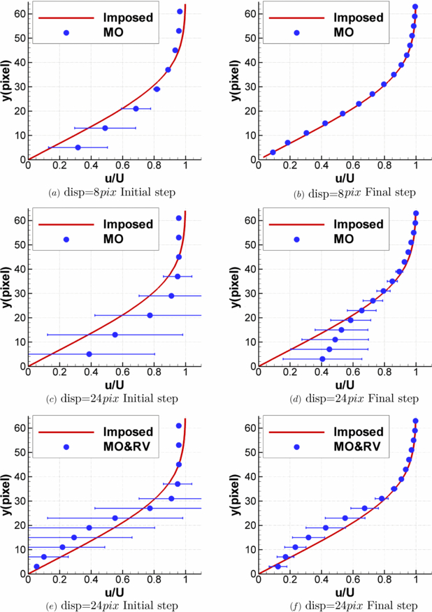
Figure 4. Estimated displacement profiles for a simulated Blasius boundary layer using the WIDIM scheme for MO. MO: wall region is masked out. : the MO interrogation was combined with vector relocation. The blue horizontal lines indicate the RMS uncertainties.

Download figure:
Standard image High-resolution imageThe evaluation errors are shown in figure 5 for various displacement gradients using WIDIM for MO. The term 'mean bias' stands for the bias of the evaluated results' mean value from the imposed value. The term 'RMS uncertainties' stands for the RMS of the evaluated results' deviations from their mean value.

Figure 5. RMS uncertainties and mean biases of the estimated displacement at the wall versus the displacement gradient using the WIDIM for MO. CP: critical point. Particle diameters were 3, 6 and 9 pixels in the flow region.
Download figure:
Standard image High-resolution imageThree different particle diameters, df, were investigated for the particles in the flow region. Each curve has a critical point (CP). For df = 3 pixels, CP is 1.1 pixels/pixels. For df = 6 or 9 pixels, CP is a little larger. Errors are rather small when the displacement gradient is smaller than CP but both the mean bias and the RMS uncertainties increase dramatically above CP and the estimated displacement eventually cannot converge to the correct result. Such results show that the WIDIM scheme is not effective on MO PIV images with very large displacement gradient near the wall.
3.2.2. WIDIM and PTV for SP and OSP with very large displacement gradients
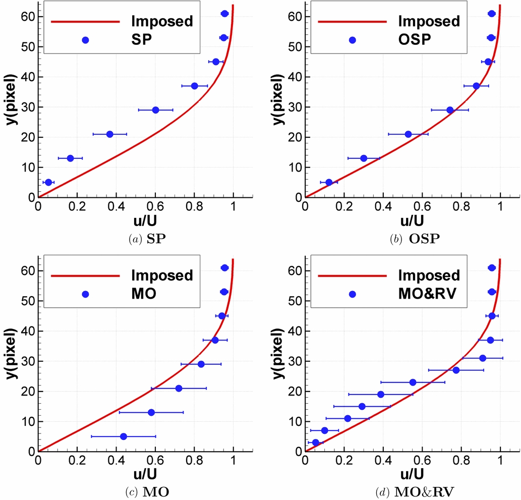
The smoothed initial estimates for SP, OSP, MO and are compared in figure 6. The free stream had a displacement of 24 pixels, corresponding to about 2.1 pixels/pixels near the wall. The addition of stationary particles introduces a reliable no-slip condition at/beyond the wall that is not possible with MO. The uncertainties, therefore, can be reduced by smoothing from both sides of the shear layer. For SP and OSP, the RMS uncertainties decrease to zero when approaching the wall. The maximum occurs in the middle of the shear layer, with a value about 50% that of MO and . The initial estimates give a proper prediction of the displacement fields and deform the PIP in the correct direction.


Figure 6. Smoothed initial estimated displacement profile for the simulated Blasius boundary layer using the WIDIM scheme. The smoothing window size was 24 pixel × 24 pixel. MO: the wall region was masked out. : the MO interrogation was combined with vector relocation. SP: the wall region was filled with stationary particles. OSP: the wall region had an optimal distribution of stationary particles. The blue horizontal lines indicate the RMS uncertainties.

Download figure:
Standard image High-resolution imageThe mean bias and RMS uncertainties are further reduced in the following interrogation result as shown in figure 7. The evaluations for all besides MO groups gradually converge to the imposed displacement profile. still have considerable mean bias error and RMS uncertainties in the middle position of the shear layer. As shown in figure 8, spurious vectors exist near the wall for MO and which interfere displacement gradient estimation and mislead the PID. For SP and OSP, the displacement velocity field is more regular with small spatial variations in the X direction for SP and smaller for OSP.


Figure 7. Final estimated displacement profile for the simulated Blasius boundary layer using WIDIM scheme. MO: the wall region is masked out. RV: the interrogation combined with vector relocation. SP: the wall region was filled with stationary particles. OSP: the wall region had an optimal distribution of stationary particles. The blue horizontal lines indicate the RMS uncertainties.
Download figure:
Standard image High-resolution image
Figure 8. Estimated instantaneous displacement field for the simulated Blasius boundary layer using WIDIM scheme. MO: the wall region is masked out. : the MO interrogation was combined with vector relocation. SP: the wall region was filled with stationary particles. OSP: the wall region had an optimal distribution of stationary particles.

Download figure:
Standard image High-resolution imageFigure 9 shows the estimated displacement using the PTV evaluation. The results are converted to a grid by a second-order polynomial fit. For SP and OSP, the mean evaluated data coincide precisely with the imposed displacement profile. The RMS uncertainties are one order of magnitude less than for MO (figure 10(a)). At some points for OSP, the RMS uncertainties approach 1% of the free stream displacement. The mean bias errors are less than 5% of the free stream displacement (figure 10(b)). Small errors still exist within 3 pixels of the interface.

Figure 9. Estimated displacement profiles for the simulated Blasius boundary layer using PTV. MO: the wall region is masked out. : the MO interrogation was combined with vector relocation. SP: the wall region was filled with stationary particles. OSP: the wall region had an optimal distribution of stationary particles. The blue horizontal lines indicate the RMS uncertainties.

Download figure:
Standard image High-resolution image
Figure 10. RMS uncertainties and mean bias of the estimated displacement near the wall of PTV.
Download figure:
Standard image High-resolution image3.2.3. Comparison of SP and OSP
Figure 11 compares the initial estimates near the wall for SP and OSP. Free stream displacement of 24 pixels is imposed in the flow region. As the window centroid approaches the wall, Ro (indicated by white arrow) increases while Rf decays (indicated by black arrow). From equation (11), the particle intensity is uniform across the interface. However, the very large displacement gradient in the flow region reduces Rf. With SP, Ro becomes much stronger than Rf even though only 1/3 of the window overlaps the wall region as shown in figure 11(d). Thus, the point d in figure 11(a) at this location is estimated to be near zero, far biased from the imposed value. By comparison, the growth of Ro is much slower in OSP. Estimate for point g in figure 11(b) at the same location is near the imposed value. Therefore, a mean bias towards zero exists on the smoothed data for SP. For OSP, the bias error is reduced to some extent, making the evaluation close to the imposed profile. In this method, the evaluation is postulated to be insensitive to the selection of parameters such as Ds. Figure 12 presents the evaluation errors of the WIDIM scheme with SP and OSP for different Ds. One interesting phenomenon is that as the displacement gradient increases, the RMS uncertainties near the wall increase somewhat but the mean bias errors decrease. For OSP, the evaluation errors are nearly stable for each value of displacement gradient. For SP, the evaluation errors are stable only when displacement gradient ⩽ 1.62 pixel/pixel; otherwise, large variations occur in the evaluation results. The mean bias and RMS uncertainties will increase when the selection of Ds is less than normal. OSP is shown to be more stable than SP when evaluating PIV images with large displacement gradients. In general, the numerical simulations show that OSP provides the best evaluations of PIV images with large displacements and displacement gradients near the wall. However, the simulations have not taken into account the out-of-plane loss of pairs, surface curvature, boundary reflection and other phenomena which are encountered in real experimental conditions. The next section further evaluates the method with the experimental data.

Figure 11. Initial estimated displacement profiles without smoothing for the simulated Blasius boundary layer for the WIDIM scheme for SP and OSP correlation maps near the wall. SP: the wall region was filled with stationary particles. OSP: the wall region had an optimal distribution of stationary particles. yc: distance from the window centroid to the wall. The blue horizontal lines indicate the RMS uncertainties. The white arrows indicate the correlation peak, Rf, from the flow region. The black arrows indicate the correlation peak Ro from the stationary particles.
Download figure:
Standard image High-resolution image
Figure 12. RMS uncertainties and mean bias for the WIDIM scheme for SP and OSP with different Ds. SP: the wall region was filled with stationary particles. OSP: the wall region had an optimal distribution of stationary particles. Ds: density of the stationary particles. Df: density of the particles in the flow region. DG: displacement gradient.
Download figure:
Standard image High-resolution image3.3. Discussion
3.3.1. Computation cost
Compared to other methods, the additional computation of the new method might only arise from the image-preprocessing steps, which consists of estimating the particle distribution parameters in the flow region and adding stationary particles in the wall region. Suppose the whole PIV recording is N × N pixels. The computational scale of estimating the particle distribution parameters is O(N2). The authors recommend that the new method had better be used in the situation when particle seeding is quasi-steady and the wall boundary is stationary. For adding stationary particles in the wall region, the computational cost mainly comes from the random generation of particle locations; however, one time is enough because of the stationary wall boundary. The flow region distribution parameters can be obtained by an average of time series.
3.3.2. Wall detection uncertainties
In order for the proposed technique to work, the detection of the wall is necessary. The effect of wall detection accuracy is necessary to be considered.
In general, the evaluation algorithm presented in this paper combines PIV with PTV. The latter one is free of the wall–fluid boundary. If the PIV prediction error near the wall is within half the distance between the flow particles, the PTV evaluation is always available. For the OSP preprocessing method, the main effect of the wall detection uncertainty is on the initial PIV evaluation. The sample points of PIV evaluation are at stationary discrete locations with the distance d = W0 · OV. Here, OV is the overlapping factor of interrogation window. For W0 = 64 pixels and OV = 75%, d = 16 pixels. Figure 13 simply describes a variation of Rf and Ro on the correlation map with the window centroidâs location. Pc is the critical location where Rf = Ro. Suppose that the detected wall location moves by δw. Correspondingly, Pc moves by δc with δc < δw. If δw < d/4 = 4 pixels, then δc < 4 pixels. Thus, no more than one evaluation sample switches its value and the created bias error is able to approach zero in the following PIV evaluation with PID. The wall detection technique presented in the paper follows the idea of Kähler et al (2006), which identifies the wall location by the symmetric line of the corresponding image pairs mirrored at the wall. The accuracy of the technique depends on the determination of particle position, the curvature of wall boundary, magnification in the optical path and so on. In the experiments, the derivation of wall location might be 1–3 pixels.

Figure 13. Variation of correlation peaks with window centroid location near the wall.
Download figure:
Standard image High-resolution imageSo far, the wall surface discussed in the paper should satisfy the condition Rc ≫ W0, with Rc being the curvature radius in pixels. The condition is applicable for the case on a relative flat surface or using high magnification imaging system. Walls with irregular features, such as a leading edge with very large curvature or small-scaled bluntness elements on the surface, are at present not considered. Such special situation is expected to be studied in the following investigation.
3.3.3. Optimum of artificial particle density and size
As mentioned before, the contribution of stationary particles to Ro comes from the parameters Isp, Ds and dp. The particle size discussed in figure 5 is of flow particles rather than stationary particles. The flow particle size may have effect on the correlation peak Rf due to the flow gradient; however, for the stationary particles, their size dp has little effect on the correlation peak Ro.
Ds is the mean density of stationary particles. As shown in figure 12, the SP method has large mean bias and RMS uncertainties when Ds is low; however, when Ds increases, the errors decrease. The reason is that there exist random fluctuations of local particle density between interrogation windows. For low Ds, the fluctuation is considerable. The OSP is relatively stable because it has effect only on the initial interrogation when the window size is large. Thus, the random fluctuations of local particle density can be neglected.
Therefore, the large Ds is, the better is the new method. The upper limit depends on the stationary particle size. The authors recommend that dp = 3 pixels and the minimum distance between the stationary particles be 5 pixels.
4. Experimental verification
4.1. Supersonic turbulent boundary layer on a flat plate
The first experiment data set is used to verify the capability of the proposed method to evaluate mean results. The experiment was performed in a small quiet supersonic wind tunnel located at the National University of Defense Technology, Hunan. The facility had a rectangular cross-section of 100 mm × 120 mm. The light sheet for illuminating the particles was 0.5 mm thick. The camera resolution was 2048 pixels × 2048 pixels, corresponding to a 60 mm × 60 mm field of view. The PIV images were obtained with a 492 m s−1 free stream velocity, which corresponds to a Reynolds number Re = 9 × 10⁶ and Mach number Ma = 3. (The local sound speed is 164 m s−1.) Nanometre size titanium dioxide particles were used to sample the flow. The particle displacement in the freestream was nearly 90 pixels. The window-correlation evaluations used 256 pixels × 256 pixels as the coarse sample, 64 pixels × 64 pixels as the medium resolution sample and PTV as the final high spatial resolution evaluation. The results of 255 pairs of recordings were averaged to give the mean result. Figure 14 shows the final PTV results with different preprocessing methods, normalized by the friction velocity uτ. The evaluated profiles for three cases in the logarithmic region are nearly the same. The wall-shear stress can be estimated from the logarithmic region of the boundary layer profile using the Clauser method (Clauser 1956) as

Here, K = 0.41 and B = 5.1. The uτ was estimated as 9.76 m s−1. Not surprisingly, the evaluations differ in the viscous sub-layer. The MO mode has non-zero displacements near the interface. The OSP evaluation gives the best description of the profile near the interface, although there are still small errors near the interface (figure 14).

Figure 14. Comparison of the mean results of PIV and PTV interrogations on the first experimental data set for a supersonic turbulent boundary layer on a flat plate. MO: masking out; RV: relocation of vector positions and OSP: optimized addition of stationary particles.
Download figure:
Standard image High-resolution image4.2. Curved subsonic laminar boundary layer on a cross-section of a slender body of revolution at high angle of attack
The second experimental data set is used to test the ability to detect velocity fluctuations in the flow near the wall. The aim of the experiment was to investigate the origin of asymmetric vortex formation over a slender body of revolution at high angle of attack. Previous studies indicated that this phenomenon is related to the asymmetric development of disturbances in the boundary layer with large adverse pressure gradients in the vicinity of the nose tip (Ericsson and Reding 1992, Bridges 2006).
The experiment was performed in the low turbulence water tunnel located at Peking University, Beijing. The facility had a rectangular cross-section of 400 mm × 400 mm. The slender body of revolution model was made of organic glass with a fineness ratio 3:1 tangent-ogive nose. The model diameter was 25 mm. The angle of attack was set at 45°. The model surface had been polished carefully by toothpaste to reduce the surface diffused reflection. The light sheet was placed perpendicular to the model axis. The light sheet thickness was estimated to be 0.2 mm. The measured cross-section was 18 mm from the model tip. The flow measurements used a histar8G type high speed CMOS camera with the Nikkor Micro 200 mm lens and a 200 mm long extension ring. The camera resolution was 1024 pixels × 1024 pixels, corresponding to a 9 mm × 9 mm field of view. The recording rate was set at 1000 Hz. The results presented here were taken at a 0.2 m s−1 free stream velocity, which corresponds to a Reynolds number based on the diameter of the model of Re = 4940. A tiny artificial disturbance was placed on the port side in the vicinity of the tip. The downstream vortex was then shed first on the port side.
A high concentration of glass beads was seeded upstream to ensure sufficient particle density in the images. The diameter of the particles is about 1–10 μm. The camera recording mode was single frame with a time interval of nearly 1 ms. Thus, the displacement of the free stream particle images in the frames was about 25 pixels. The evaluations were conducted with a 64 pixels × 64 pixels coarse sample and 32 pixels × 32 pixels medium resolution sample and finally PTV to achieve high spatial resolution.
Figure 15 shows the mean velocity profile at azimuth 45° on the port side, summarized from 100 instantaneous results. The behaviours of different cases were the same as in the first ensemble. The OSP evaluation gives the best description of the profile near the interface. There are some differences from the simulations (Moore 1951), because some conditions such as angle of attack and the pressure gradient, were different.

Figure 15. Comparison of the mean results of PIV and PTV interrogations on the second experimental data set for a curved subsonic laminar boundary layer on a cross-section of a slender body of revolution at high angle of attack. MO: masking out; reMO: relocation of vector's position; OSP: optimized addition of stationary particles.
Download figure:
Standard image High-resolution imageHigh speed PIV system was used to enhance the instantaneous measurements accuracy. The instantaneous results were summarized by every ten results so that some interferences, e.g. the local unsteady and non-uniform particle image distributions, were reduced. Figure 16 shows the velocity fluctuations' distribution, which are mainly in the thin shear layer near the interface with the maximum value less than 0.015 U. The fluctuations on the port side are larger than on the starboard side. As mentioned before, an artificial disturbance was placed on the port side ahead of the measured cross-section. The evaluated result is in agreement with the reality.

Figure 16. Statistical results of the second experimental data set for a curved subsonic laminar boundary layer on a cross-section of a slender body of revolution at high angle of attack. The lee side of the field is cut off because of lack of particle images. (a) Mean velocity field. (b) RMS of fluctuations distribution.
Download figure:
Standard image High-resolution image4.3. Hypersonic boundary layer in transition on the symmetric plane of a flared cone at zero angle of attack
The third experimental data set is used to test the capability of the proposed method to explore small flow structures near the interface. In the recent years, the existence of second-mode waves and their significance to the transition of hypersonic boundary layer (figure 17) have been investigated theoretically, experimentally and numerically by many researchers (Mack 1984, Schneider 2004, Zhong and Wang 2012). However, the direct instantaneous PIV measurement is still a challenge. The third ensemble of experimental data was obtained in the newly established Mach 6 quiet wind tunnel (M6QT) of Peking University. The free stream velocity was around 800 m s−1, corresponding to unit Reynolds number Re = 5.8 × 10⁶ /m and Mach number Mach = 6. The PIV time interval was more than 1 μs which made particle displacements between frames as high as 2 mm, the same order of the wave length of second-mode waves. The corresponding displacements on the recordings were about 100 pixels. Meanwhile, the ratio of in-plane particle pair was less than 50%, which led to a small SNR in correlation map.

Figure 17. Flow visualization of transition induced by the second-mode wave in the hypersonic boundary layer.
Download figure:
Standard image High-resolution imageThe images were rotated horizontally at first and preprocessed by the OSP method. Then they were evaluated in sum-of-correlation mode. The evaluations were conducted with a 256 pixels × 256 pixels coarse sample and then 128 pixels × 128 pixels medium resolution sample to capture the mean displacements. Based on the mean result, the instantaneous recordings were then evaluated with 64 pixels × 64 pixels small sample. Smaller sample is unavailable because of the low SNR. Figure 18 compares the results between the and the OSP method. It can be seen that the new method has successfully extracted the small flow structures of the second-mode wave in the hypersonic boundary layer from PIV images with low SNR when the traditional method was not successful. When the transition occurred, a series of small vortex was created in the hypersonic boundary layer by the wave–vorticity interaction. The inner structure of the vortex is shown in figure 18(b). The measured wavelength coincides with the flow visualization and pressure measurement (Zhang et al 2013). Such result is obtained for the first time, which proves the capability of the current method to explore the near-wall small flow structures in the high speed flow with low SNR.


Figure 18. Comparison of the instantaneous results of a PIV interrogation on the third experimental data set for the transition induced by the second-mode wave in the hypersonic boundary layer. (a) velocity field. (b) OSP velocity field. (c) OSP streamlines. (d) OSP vorticity field. MO: the wall region is masked out. : the MO interrogation was combined with vector relocation. OSP: the wall region had an optimal distribution of stationary particles.


Download figure:
Standard image High-resolution image
5. Conclusion
The conventional WIDIM scheme is a powerful algorithm to estimate the high shear flow. However, when the method encounters very large in-plane displacements and displacement gradients near the interface, it will suffer large distortions in the mean and instantaneous evaluations. In this paper, an algorithm based on a new image-preprocessing method has been presented. Several image-preprocessing methods have been assessed by means of Monte Carlo simulations and real experimental data. These methods include conventional digital mask technique (MO) with or without vector relocation (RV); addition of stationary particles with uniform intensity in the wall region (SP) or its optimized arrangement (OSP). It can be concluded that:
- (i)For the MO method, the displacement gradient has a critical point (CP) for the WIDIM evaluation. When the displacement gradient is below 1.2 pixel/pixel, the evaluation errors are rather small. The RMS uncertainties are smaller than 1% of the free stream. When the displacement gradient becomes larger, the errors will grow dramatically. The RMS uncertainties can increase by more than one order of magnitudes when the displacement gradient is more than 1.5 pixel/pixel. In this case, the evaluation cannot converge to the correct result.
- (ii)For the SP or OSP method, the initial estimate can be smoothed from both side of the shear layer so that it becomes more reliable. The subsequent interrogations then converge to the correct result and provide an adequate prediction for the PTV evaluation. Compared to the MO method, the RMS uncertainties and the mean bias are reduced by one order of magnitude.
- (iii)Compared to the SP method, the OSP method is more stable with different image-preprocessing parameters. Under real experimental conditions, the OSP method was shown to be robust and accurate in evaluating the flow near the interface with very large displacements and displacement gradients. The algorithm has successfully extracted the small flow structures of the second-mode wave in the hypersonic boundary layer from PIV images with low SNR when the traditional method was not successful.
There is still a lot of room for improvements in the current method. For example, the square window shape is not the optimum choice for interrogation near the interface. In the future works, an integrated methodology considering preprocessing, evaluation algorithm and postprocessing will be investigated.
Acknowledgments
This work was supported by the National Natural Science Foundation of China under grant no 109103010062. This work was also supported by the National Climb-B Plan under grant no 2009CB724100 and the National Natural Science Funds for Distinguished Young Scholar group under grant no 10921202. The flow visualization and PIV images of supersonic turbulent boundary layer on a flat plate were kindly provided by Qing Tang from the College of Engineering, Peking University.