

Abstract
Thermal convective air flows are of great relevance in fundamental studies and technical applications such as heat exchangers or indoor ventilation. Since these kinds of flow are driven by temperature gradients, simultaneous measurements of instantaneous velocity and temperature fields are highly desirable. A possible solution is the combination of particle image velocimetry (PIV) and particle image thermography (PIT) using thermochromic liquid crystals (TLCs) as tracer particles. While combined PIV and PIT is already state of the art for measurements in liquids, this is not yet the case for gas flows. In this study we address the adaptation of the measuring technique to gaseous fluids with respect to the generation of the tracer particles, the particle illumination and the image filtering process. Results of the simultaneous PIV/PIT stemming from application to a fluid system with continuous air exchange are presented. The measurements were conducted in a cuboidal convection sample with air in- and outlet at a Rayleigh number Ra ≈ 9.0 × 10⁷. They prove the feasibility of the method by providing absolute and relative temperature accuracies of σT = 0.19 K and σΔT = 0.06 K, respectively. Further open issues that have to be addressed in order to mature the technique are identified.
Export citation and abstract BibTeX RIS
1. Introduction
Thermal convective flows occur in technical applications such as heat exchangers [1] or indoor climatization [2] and are of great interest in fundamental studies too. Since these flows are thermally driven, simultaneous measurements of the instantaneous velocity and temperature fields are highly desirable, e.g., to study the dynamics of thermal plumes and their influence on the local and global heat transfer in thermal and mixed convection, or to allow for profound statements to issues like passenger comfort and heat transport processes in aircraft cabins [3, 4]. Possible measurement techniques in liquids, e.g. water, are molecular tagging velocimetry and thermometry [5, 6] or the combination of laser induced fluorescence (LIF) and particle image velocimetry (PIV) [7]. Another established technique in liquids is the combination of particle image thermography (PIT) and PIV with thermochromic liquid crystals (TLCs) as tracer particles [8–11]. Thereby, this combined technique is based on the well-known PIV algorithms for velocimetry [12] and the special behaviour of the TLCs in reflecting light with different wavelengths when having different temperatures for the thermometry [13, 14]. Details about the measurement technique can be found in the review papers of Smith et al [13] and Dabiri [14] as well as in Tropea et al [15] (see chapter 7.1). However, the above cited references address combined velocity and temperature measurements in liquids only. Ahlers et al [16] and Puthenveettil et al [17] showed that flow properties such as large-scale structures, the Nusselt number, i.e. the heat transport and the length of near-wall plumes, depend on the Prandtl number. Since air flows with a Prandtl number of Pr ≈ 0.7 are found not only in many technical applications, e.g. indoor climatization [2], but also in more fundamental thermal convection problems, the development of a combined velocity and temperature measurement technique for gaseous, especially air, flows is very desirable. Thus, the intention of our work is the combination of PIT and PIV using TLCs as tracer particles in air flows. In particular, we are interested in systems with continuous fluid exchange, such as the climatization problems mentioned above, which pose some additional challenges to the measurement technique.
The feasibility of combined PIT and PIV for pure thermal convection has already been demonstrated in a cubical Rayleigh–Bénard cell with air as the working fluid [18, 19]. In these measurements the TLC tracer particles were sprayed into the cubical cell which was closed after the particle injection. After a short settling time, the images for PIT and PIV were recorded with two cameras, a grey level double shutter camera (Pixelfly QE, ©PCO) and a commercial digital reflex camera (D70s, ©NIKON). This setup allowed first measurements in thermally driven air flows in closed systems with no air exchange.
Other possibilities for acquiring the temperature and the velocity field in air flows are the combination of LIF and PIV [7] or the acoustic tomographic imaging of the temperature and flow field [20]. Nevertheless, these promising techniques are either just proposed and not yet accomplished (LIF/PIV), or reveal only very poor resolution so far (acoustic tomographic imaging).
Furthermore, Fujisawa and Hashizume [21] have suggested that highly accurate measurements of the velocity can only be carried out using additional tracer particles in order to satisfy the condition for PIV analysis. Whether and to what extent this claim holds for the adaptation of this combined measurement technique to air flows will be analysed in the near future by a comparison of conventional PIV results with those acquired with white light and TLC tracer particles.
This paper is intended as a step towards simultaneous measurements of instantaneous temperature and velocity fields in air flows in open systems with air exchange using TLCs. It is structured as follows: section 2 first reviews some of the fundamentals of TLCs, then discusses the new achievements in particle generation, their illumination and finally the issues of the image filtering process. This section is followed by a paragraph on the application of the novel measurement technique to a convection experiment. A summary and conclusion including an outlook is given at the end of the article.
2. General considerations of combined PIT and PIV
The general requirements that must be fulfilled to apply TLCs as tracer particles in air flows for combined PIT and PIV are the following. First, in order to conduct PIT, they have to provide a temperature-dependent reflection of different wavelengths with a short temperature response time. Second, for accurate PIV, the tracer particles must possess good following behaviour, a high light scattering efficiency and a long lifetime. Additionally, for systems with continuous fluid exchange, the tracer particles need to be continuously produced at a high rate. Furthermore, it has to be considered that the colour play of the TLCs, which is exploited in PIT to locally detect the fluid temperatures, not only depends on the temperature but also on, e.g., the angle between the incident illumination and line of view, the background light, as well as the size and the age of the droplets. Consequently, a spatially resolved calibration is needed for high precision measurements, and TLC particles with a narrow size distribution have to be generated. While all of the above discussed issues are addressed in our ongoing study, this paper focuses on the recent progress in particle illumination and characterization as well as image processing.
2.1. Fundamentals of thermochromic liquid crystals
Based on the review papers of Smith et al [13] and Dabiri [14], some of the fundamentals of TLCs, especially some of the colour-dependent parameters, are described in the following. It is well-known that the colour of a TLC droplet depends not only on its temperature but also on, e.g., the angle between the incident illumination and line of view, the background light and the age of the droplet. Due to the angular dependence, a local calibration provides far better accuracy than a global calibration. Another important parameter is the size of the droplets. Hence, a major requirement is that the produced particles have a sharp size distribution. In this respect the minimal/maximal possible size of the TLCs, which depends on two factors, must be detected. On one hand the TLCs must maintain their temperature-dependent reflection of different wavelengths (the play of colours), i.e. they must be as large as possible, and on the other hand, they need the best possible following characteristics, i.e. they must be as small as possible.
From previous studies by Czapp [18] and investigations of the colour play of the crystal as a function of the particle generator settings, we know that the diameter of the TLCs should be of the order of 10 μm. An estimate of the reaction time of the TLCs to temperature changes, the following behaviour and the sinking velocity is given in Czapp [18] and Raffel et al [12]. There, the reaction time based on the heat transport from the fluid to crystal via convection (τα) is estimated as  using Nu = 2 for very creeping flows. Here, α is the heat transmission coefficient. The other possible heat transfer mechanism from the fluid to the crystal is heat radiation (τσ), which can be approximated using the Stefan–Boltzmann law and the emissivity
  = 1. Once heat is transferred from the fluid to the crystal, or vice versa, the surrounding is colder than the crystal. Thus, the crystal itself must transport the heat to its interior by heat conduction (τλ), which can be estimated based on the heat conductivity of the crystal λp. Finally, the helical structure of the crystal, i.e. the colour of the crystal, must change according to the temperature of the crystal. Since this relaxation time τrelax is hard to estimate we refer to the value 100 ms for cholesteryl ester and 1–10 ms for chiral nematic crystals published in [22–25]. Thus, based on the above discussed assumptions, one obtains the following estimates for the relevant reaction times for the colour change of a TLC particle with a diameter dp = 10 μm:
with the heat capacity per volume of Cp, the Stefan–Boltzmann constant σ and the ambient temperature T. The above shown three orders of magnitude higher reaction times of the radiative heat transport to the particle (τσ) are negligible compared to the heat transport via convection (τα). Contrarily, the time constant for the internal heat conduction within the particle (τλ) is like that of τα of the order of milliseconds as well. Another important time constant is the time that the TLC needs to change its colour after having changed its temperature τrelax. For thin layers of chiral nematic crystals, which is the crystal type we use in our experiments, values in the range 1–10 ms are reported for τrelax in the literature [22–25]. Although the lateral dimensions of the TLCs might affect τrelax, the values for small droplets of chiral nematic crystals are similar. Dabiri [14] reports response times for TLC particles from Hallcrest with a diameter of 10 μm of 1–4 ms. Tropea et al [15] give a response time of 3–10 ms for TLC tracer particles with diameters of 20–50 μm. However, much larger values of up to 100 milliseconds are reported for another crystal type, i.e. cholesteryl ester (cholesteric) crystals [22–24]. According to the discussion above we expect the overall thermal response time τt to be below 10 ms for our chiral nematic crystals (Hallcrest, R20C6W) with a mean diameter of approx 10 μm. It is a function of the processes discussed above, some of which proceed in parallel while others take place consecutively. However, our analysis revealed the relaxation time as the limiting time scale, while direct measurements of τrelax of dispersed TLC particles in air have not been reported so far and constitute an open issue. However, in spite of the fast response time compared to conventional temperature sensors, precise temperature measurements are possible only if the TLC particles are able to adapt their temperature on time scales comparable to that of the local convective velocity and the spatial resolution of the measurement. To quantify this, we estimate the maximal travelled distance δmin = τt · umax during the reaction time τt, which ought to be smaller than the minimum of the interrogation window size and the size of the smallest coherent structures, i.e. approximately 10 times the Kolmogorov length ηK [26]:
In our measurements, the maximal fluid velocity is umax ≈ 0.1 m s−1, thus δmin ≈ 10−3 m, while 10 · ηK ≈ 10−2 m (for Ra ≈ 108 and Pr ≈ 0.7) [26] and the interrogation window size amounts to dint. window ≈ 5 × 10⁻³ m. Hence, the thermal reaction time is short enough for the here considered flows.
An overview of the parameter range in which the technique is applicable according to the above discussed limitations is depicted in figure 1. The dark grey shaded triangle in figure 1, in which the measurement technique can be applied, reflects that the spatial resolution not only decreases with increasing velocity but also crucially depends on the reaction time, which lies between 1 and 10 ms. The region of resolvable spatial fluctuations depending on the maximal fluid velocity u is highlighted in light and dark grey for τt = 1 ms and τt = 10 ms, respectively. For the interrogation size of the measurements presented below, which is marked as the black dot in figure 1, the response time of τt = 10 ms is small enough. However, it must be noted that if this is not the case, backtracing of the particle positions using the measured velocity field with sophisticated tracing algorithms allows enlargement of the parameter range in figure 1 in which the measurement technique can be applied.
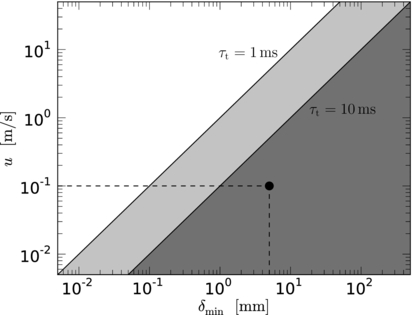
Figure 1. Parameter range dependent on the spatial resolution depending on the thermal reaction time of the TLCs and the maximal fluid velocity with applicability range of the measurement technique shaded in dark grey. The values of our measurement are marked with the black dot.
Download figure:
Standard image High-resolution imageOther important parameters, which might limit the accuracy, are the mechanical reaction time τm and the sinking velocity due to gravity vg. They can be estimated (following Raffel et al [12]) assuming Stokes friction:
using the particle density ρp ≈ 1.01 × 10³ kg m−3 (ρTLC = 1.00–1.02 × 10³ kg m−3 given by Hallcrest for the unencapsulated TLCs used by us), the gravitational acceleration gas well as the density ρ ≈ 1.2 kg m−3 and the dynamic viscosity η ≈ 1.8 × 10⁻⁵ of air at 20 °C. Although this sinking velocity is lowered by the Brownian motion, it is still a limiting factor for the total measurement time without supplying new particles and the accuracy of the velocity measurement. Again, based on the assumption of Stokes, Raffel et al [12] describe the following behaviour of the smallest particles while travelling through a shock wave:
with the velocity of the particle vp(t) and the velocity of the surrounding fluid v∞. These estimates result for a dp = 10 μm TLC particle in an air flow in a time of t ⩽ 3 ms that the particle needs to reach 99% of the fluid velocity. Thus, TLC particles with dp ⩽ 10 μm follow rather slow fluid flows almost instantaneously.
To calculate the temperature from the colour of the TLC particles, a transformation of the colour space must be applied. For the TLC particles used with this specific diameter, a calibration of the temperature-dependent hue value [14] has to be performed, so that a temperature accuracy better than ±0.3 K is achieved. Thereby the hue is, besides saturation and value or saturation and lightness, one of the three parameters of the hue/saturation/value (HSV) or hue/lightness/saturation (HLS) colour space, respectively. For graphical representations of the colour spaces, see figure 2. The parameter value is the only non-obvious parameter, and can be understood as the brightness (or darkness) value of the colour with V = 0 being black and V = 1 being the pure colour. The hue saturation intensity colour space is another possible colour space which can be used for the calibration of temperatures to colours. Its difference from the HLS colour space is only the third parameter: lightness is the relative light intensity and intensity is the absolute one. Using either one of these does not matter much. For completeness it should be noted that the hue saturation brightness (HSB) colour space, which some of the literature refers to, is exactly the same as the HSV colour space, only naming the parameter, more obviously, brightness instead of value. Nevertheless, in the following, we will use the name HSV instead of HSB because it is the more common expression.

Figure 2. Representations of (a) the HSV and (b) the HLS colour space.
Download figure:
Standard image High-resolution imageThe hue value h can be calculated from the RGB values (red: r, green: g, blue: b) [27] by:
The parameters saturation and lightness, intensity or value can be used to correct artefacts like black or white pixels of the image and for the filtering process which is needed for the separation of the particles from the background. A possible realization of this process is described in section 2.4. All colour information needed to calculate the temperature is expressed with the single parameter hue, hence this parameter is used to calculate the temperature from the colour image.
2.2. Generation of tracer particles
For the production of tiny unencapsulated TLC particles, a generator is needed that fulfils the following requirements. Firstly, to investigate systems with air exchange, continuous production of the particles must be realized. Secondly, the particles have to exhibit a sharp size distribution in order to allow for well-defined colour play and finally, the mean particle size, however, should be adjustable by the operational parameters of the generator in order to allow matching of the size-dependent particle colour play to the actual measurement. The final particles must, on one hand, maintain their temperature-dependent reflection of different wavelengths (the play of colours), i.e. they must be as large as possible. On the other hand, they need the best possible following characteristics, i.e. they must be as small as possible.
While in previous studies, particle generation based on the Rayleigh instability [28], which potentially provides some of the above mentioned requirements, was employed [19], two different generators have been tested. One is based on an air-atomizing nozzle (0.25 mm nozzle diameter, liquid nozzle: PF1050, air nozzle: PA64, ©Spraying Systems) and the other one is an airbrush system (0.3 mm nozzle diameter). An inverted grey scale image of the particle jet produced by the airbrush system is presented in figure 3. Both generators provide a particle production rate that is sufficient for measurements on the square meter scale. To generate the tracer particles, the TLC mixture is first dissolved in isopropyl alcohol. In the second step, the mixture is atomized by the generator. After evaporation of the isopropyl alcohol from the atomized droplets, atomized TLC tracers remain. However, the resulting particles do not have a monodisperse size distribution, see figure 4(a) and (b). Due to the above mentioned aspects, it is almost impossible to measure the TLC particle size directly. Therefore we used water instead of the TLC mixture and measured the particle size distribution produced with the generators by applying phase Doppler anemometry (PDA). The diameter statistics of the generated water droplets for both generators at their working points are presented in figure 4. All droplet sizes were measured with a PDA system assuming spherical droplets. The particle generators used provide a sufficient number of particles with the desired density and size distribution and are therefore well suited for simultaneous PIT/PIV investigations. A further analysis of the particle diameter distribution of the generators revealed that the airbrush system provides droplets whose diameters follow a log-normal distribution, see the Gaussian curve on a logarithmic x-axis (inlay of figure 4(a)). For the air-atomizing nozzle, no such simple particle distribution was obtained. The semi-logarithmic plot (inlay of figure 4(b)) reveals that there is a rather high proportion of large particles. These particle statistics underline that the airbrush system provides a sharper size distribution and, therefore, appears to be more suitable for our purposes. Nevertheless, more development work can be performed with respect to the generation of TLC particles, to further optimize, e.g. the dispersity of the generated particles.

Figure 3. Inverted greyscale image of the particle jet produced by the airbrush system.
Download figure:
Standard image High-resolution image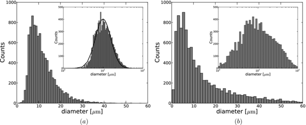
Figure 4. Diameter statistics of generated water droplets for both particle generators: (a) airbrush system, (b) air-atomizing nozzle at pfluid = 0.2 bar and pair = 0.3 bar, inlays: logarithmic x-axes.
Download figure:
Standard image High-resolution imageIn our experiments, the mass mixing ratio between the TLC mixture and isopropyl alcohol was set to 1: 2 or 1: 1, eventually resulting in a TLC particle size smaller than the produced droplets by a factor of approximately 1.4 or 1.3 in diameter, respectively. Of course, variation of the mixing ratio opens up another possibility to vary the TLC tracer particle size.
For the results presented in this paper, we used the airbrush system and a mixing ratio of 1: 1 for the particle generation. The size of most of the produced TLC-isopropyl alcohol droplets turned out to be approximately 10 μm, see figure 4(a). Thus, the TLC particle diameter should be in the range of dp ≈ 7 μm. The particles produced with this combination of generator and mixing ratio, led to the so far most convincing results in simultaneous PIV and PIT. Please note that according to the assumptions given by Raffel et al [12], discussed above, the mechanical reaction time until the particles reach 99% of the fluid velocity is in the order of τm ≈ 1.5 ms. For the rather slow flows considered here, the particles are assumed to follow the surrounding fluid instantaneously.
2.3. White light sheet
One of the main components in a simultaneous PIT/PIV setup is the white light sheet. For high quality PIV measurements, it should provide an intensity that is high enough and a collimation that is good enough to allow sharp imaging of single tracer particles. This implies also that the pulses of the light source must be short enough to not smear the particle images. Furthermore, the flashing frequency should be as high as possible, to achieve the best possible time resolution as well.
The white light sheet employed in our measurements is based on light emitting diodes (LEDs) and was specially developed for this purpose. The LEDs have the advantages of low cost, easy handling and good luminous efficiency. However, their drawbacks are the low coherence and high divergence of the emitted light and their finite size, i.e. they cannot be considered as point sources. A successful implementation of LEDs for PIV investigations was already reported in Willert et al [29]. Due to the need for high light intensity, white colour and good focusability at the same time in our application, we developed a light sheet source based on 60 ©OSRAM Platinum Dragon LEDs, LW W5SN-KYLY-JKQL, which are arranged in a one-dimensional array on a printed circuit board. Each single LED is equipped with a clip-on lens (©SHOWIN Clip-On Lens for Osram GD+ LED) in order to reduce the angle of radiation from approximately 120° to approximately 15°. Another main advantage of the applied clip-on optics is their small spatial extension, which is just a bit larger than the LEDs, allowing the achievement of a spatial density of 11.6 LEDs per 10 cm. The one-dimensional array of LEDs is used in combination with a slit aperture and a cylindrical lens. By adjusting the distances between the different elements, one can manipulate the brightness and divergence of the produced light sheet. A sketch of the light sheet optics is shown in figure 5.

Figure 5. Sketch of the new developed white light sheet optics, including the LED array, the clip-on optics and a combination of a slit aperture and a cylindrical lens for the formation of the light sheet.
Download figure:
Standard image High-resolution imageEach of the white light emitting LEDs has a luminous flux of 191 lm at a forward current of 1 A [30]. PIV investigations require a pulsed light source, this implies that the LEDs can be operated at an increased forward current of 3.3 A. For reasonable PIV results in thermal convection at Pr ≈ 0.7 and moderate Ra numbers, a pulse length equal to or shorter than approximately 1 ms is sufficiently short. The duration of the light pulses and the time delay between the first and the second pulse for PIV can be controlled with an external trigger unit using TTL signals. The time response of the light source to a double pulse TTL trigger signal was measured using a photodiode, placed in the light sheet, and a oscilloscope. For the characterization of the light source only, the delay between the two pulses was set to τ = 5 ms and the duration of each pulse to 1 ms. While the pulse duration is kept at 1 ms during our actual experimental investigations, the delay time is adjusted to τ = 16 ms in order to get a maximal pixel displacement in the order of Δx ≈ 10 px. Figure 6 shows the time traces of the light sheet output and the trigger pulse. Thereby, figure 6(a) depicts both pulses necessary for PIV investigations, and (b) sketches a magnification of just one pulse, to show the reaction of the light output on a trigger signal. The rise and fall times of the light output are 44 μs and 63 μs, respectively.
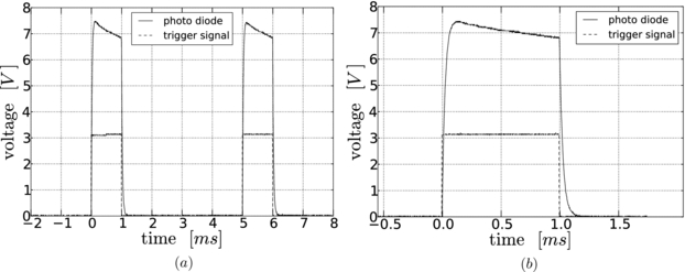
Figure 6. Time trace of light emission as detected by a photodiode (—) as response to a TTL trigger signal (−−): (a) 1 ms light pulse duration and a time delay between the first and the second trigger signal of 5 ms, (b) magnification of one of the two pulses depicted in (a).
Download figure:
Standard image High-resolution imageThe recorded pulse duration of 1 ms is sufficiently short for investigation of rather slow flows, e.g. indoor climatization, but may not be applicable for high flow velocities (also depending on the used camera and lens system). At high flow velocities, such a long pulse duration will lead to elliptically stretched rather than sharp circular images of the tracer particles, and therefore will lead to decreasing accuracy of the velocity evaluation. We also tested a shorter light pulse length of 0.5 ms, which makes it possible to measure faster flows as well. Due to a better signal to noise ratio and no drawbacks in the quality of the particle images, we used a pulse length of 1 ms for the study presented here. It should be noted that τ = 5 ms was fixed for the characterization of the light source, only. During the measurements, τ was adjusted to get pixel displacement values which are suitable for the PIV interrogation, see section 3.2.
Figure 7(a) presents intensity profiles of the lightsheet, which were measured using a photodiode mounted onto a traverse stage. For all presented distances (100 mm ⩽ x ⩽ 500 mm) from the front lens of the light sheet optics, a Gaussian profile was found. To further characterize the light sheet, the maximal values of the photo voltage as well as the full width of the profiles at half maximum (fwhm) are presented in figure 7(b) for distances from 50 to 1000 mm. One finds that for x ⩽ 500 mm the maximal photo voltage (i.e. the luminous intensity of the light sheet) drops only by 25%, while the thickness in terms of fwhm is always less than 10 mm. For larger distances, the maximal photo voltage drops rather quickly, to approximately 30% of its maximum, and the light sheet thickness increases up to 18 mm at x = 1000 mm.

Figure 7. (a) Intensity profiles of the lightsheet (at half height of the lightsheet) and (b) maximal intensity and full width at half maximum (fwhm) for various distances from the front lens, measured using a photodiode.
Download figure:
Standard image High-resolution imageThus, summarizing, we can state that the developed white light sheet optics produces a light sheet with a thickness (fwhm) of approximately 9 mm, very low divergence and rather homogeneous illumination over a distance of 500 mm.
The repetition rate is, at present, set to 4 Hz and in our investigations limited by the cameras used rather than by the light sheet optics. It is much higher than the repetition rate of approximately 1/5 Hz that Czapp [31] was able to realize. Furthermore, the new frequency of 4 Hz allows for well time-resolved studies of rather slow processes, e.g. indoor climatization or convection driven flows at low and moderate Rayleigh numbers in which we are interested.
2.4. Image filtering process
A characteristic difficulty of PIT of air flows arises from the large difference of index of refraction between fluid and particle. While this is advantageous for parallel PIV measurements, the high amount of Mie-scattered white light tends to overcast the colour information of the inelastically scattered light. Precise PIT measurements thus require special attention during image processing in order to separate the temperature-dependent colour information from the background noise. In order to keep the amount of scattered white light to a minimum, the PIT camera was positioned at an angle of approximately 45° in the backward direction, which already reduces the background significantly. Such a camera setup for PIV leads to perspective errors associated with the out of plane velocity component. While the backward position of the colour camera is essential to receive sufficient image quality for PIT, the viewing angle of the PIV camera can be chosen independently. In the current study the PIV camera has been installed viewing slightly into backward scattering for practical reasons. However, in future measurements the PIV camera can be operated perpendicular to the field of view as well, while the colour camera is maintained in the backward direction, as long as the optical accessibility of the setup allows it.
The images for both PIV and PIT are recorded simultaneously with two Pixelfly (©PCO) cameras, one grey level double shutter and one colour camera. The double shutter camera is used for the well-known PIV evaluation (see e.g. [12]). For the temperature measurements the colour camera is used. This camera records red/green/blue (RGB) images with a Bayer filter (step 1 in figure 8). Both images are deskewed and overlapped using calibration grids and are projecting tools similar to those used for stereoscopic PIV.

Figure 8. Sketch of the image filtering process. Step 1: recorded RGB image, step 2: decomposed HLS/HSV image, step 3: generation of the mask using L and S or S and V, step 4: application of the mask to H, step 5: calculation of the local temperatures using hue–temperature calibration functions.
Download figure:
Standard image High-resolution imageSince no neutral sunlight is used for illumination, a specific white balance is fundamental for acquiring realistic and reproducible colours. Therefore, we use a neutral greycard which has a remission of light that is independent of the wavelength of the incident light. Such a card is well-known in photography. It allows the determination of a reference value for each setup, in particular for a specific arrangement of the illumination, and thus to choose the right white balance which guarantees a neutral colour and reproducibility.
For filtering and temperature analysis, these images are converted into the HSV or the HLS colour space (step 2 in figure 8). Due to the finite width of the particle size distribution, the recorded images reveal a rather high amount of background noise. In order to take only the colourful particles into account, a threshold for the value (HSV) is used in order to filter the hue values (step 3 and 4). Different filter algorithms could also be based on the saturation (HSV or HLS) or the lightness (HLS). Finally, the local temperatures can be calculated using hue–temperature calibration functions (step 5).
The main challenge is to identify those pixels which are neither background noise, nor small particles scattering white light. This can be done in different colour spaces. For a realization in the HLS colour space, only those pixels should be taken into account that have a high saturation and a lightness in the range of < L < 1 − with > 0. In the HSV colour space, both parameters saturation and value must be above a certain threshold. However, we could get rather good results by using a local filter which is just based on the value parameter of the HSV colour space. Therefore, we will focus on the HSV colour space and in the following all given parameters, hue, saturation and value, will correspond to this colour space.
As an example, a synthetic image with different coloured particles and background noise is generated. It is shown in figure 9(a). The background noise is set to 0.1 ∈ [0, 1], the particles with a size of 3 × 3 px are placed on top of the noise and have linearly decreasing intensity from left to right of 0.9 to 0. Thus, close to the right side of the image the particles vanish within the noise. Such a configuration is chosen to see how robust the filtering algorithm is with respect to the signal to noise ratio. The colours of the particles are red at the top, then passing to yellow, green, blue and purple, until they become red at the bottom again. Therefore, the hue increases from top to bottom from H = 0 to H = 1.

Figure 9. Filtering process of the raw images for the separation of the particles from the background noise: (a) synthetic colourful particle image (RGB), (b) hue channel (in HSV colourspace), (c) mean hue value in 16 × 16 px interrogation windows, (d) value channel (in HSV colourspace), (e) hue versus value for a 16 × 16 px interrogation window, box marks those pixels with highest four value levels which are used for the hue calculation within this window, (f) final hue image in 16 × 16 px interrogation windows after filtering using a threshold in the value channel, (g) colour scale for images (b), (c) and (f).
Download figure:
Standard image High-resolution imageFigure 9(b) presents the pixelwise calculated hue map of the test image. One finds a random distribution of all hue values, clearly showing that the hue cannot directly be used for the calculation of the colour and therefore the temperature distribution.
The next possible step is to apply a median filter. The result for a 16 × 16 px median filter is shown in figure 9(c). The tendency of increasing hue from top to bottom is visible now, nevertheless all mean hue values are in the vicinity of H = 0.5. This is caused by the impact of the background noise with random hue values and clearly shows that an image which has more background than particles cannot be simply evaluated by calculating the mean hue within interrogation windows.
The idea is to use interrogation windows again, but to take only those pixels into the calculation of the mean hue value for this interrogation window that are not background noise. Due to slightly inhomogeneous illumination in almost all experimental setups, we applied such a filter with a local rather than a global threshold for the identification of particles. Therefore, we chose the V value, i.e. the brightness (see figure 9(d)), of the colour image and localize those pixels where the value of V has increased from the background level. Within each interrogation window, we take only those pixels into account for the calculation of the mean hue for the whole interrogation window, where the highest V-values are located. To clarify this procedure, figure 9(e) shows a scatter plot of hue versus V-value for a 16 × 16 px interrogation window. For low values of V (V ≲ 0.1), one finds all H ∈ [0, 1], but for high values of V, only a rather sharp hue distribution appears. We identify those pixels as the particles and the rest as the background noise. For the calculation of the mean hue, we take into account only the pixels with the highest value of V, which are marked with a box; in this example the threshold was set to four. Both the size of the interrogation windows as well as the threshold for how many pixels should be taken into account must be adjusted to the particle density of the image.
Applying this procedure to the synthetic image results in figure 9(f). One can see three things: firstly, the hue gradient from almost H = 0 at the top to almost H = 1 at the bottom can be reproduced. Secondly, even at a very low signal to noise ratio, on the right side of the image, the algorithm reproduces the hue values correctly. Thirdly, in red regions where H ≈ 0 or H ≈ 1, some errors are produced due to fact the hue is periodic and that a pure red colour is either H = 0 or H = 1. However, for the calibration of the liquid crystals this fact should not be bothersome, because the liquid crystals turn from red to yellow and green to blue until they become colourless again, meaning that H ≈ 1 will not appear using liquid crystals.
Although filtering can be realized in a similar way in the HLS colour space, filtering with the V-value in the HSV colour space yields good results for almost all investigated particle images so far, so we concentrate on this technique for now.
2.5. Dynamic calibration
To obtain the absolute temperature information from the hue values, a hue–temperature calibration must be conducted. The calibration function found is only valid for the specific setup, i.e. only for the specific arrangement of cameras and light-sheet optics as well as for the crystal type and the particle generator used. Typically, during periods of stable layering of the temperatures, the different hue values and the corresponding temperatures are recorded. Due to the difficulty of generating these stable temperatures within our geometry and due to the high time effort of this calibration technique, we decided to apply, as a fast approach, a dynamic calibration to correlate the recorded hue values to the absolute temperatures. The main advantage is the rapidity of the calibration process. Therefore, a very quickly reacting, precisely calibrated glassbed NLC thermistor with a diameter of only 400 μm is placed within the measurement plane. Using this thermistor, which is calibrated with an accuracy of σT, therm. = 0.05 K, the temperatures are recorded at a high frequency (compared to the recording frequency of the PIT/PIV images) of approximately 13 Hz. For the hue–temperature calibration, the hue values are evaluated as described in the previous section and those hue values recorded next to the position of the thermistor are correlated to the temperatures. This results in time series for hue and temperature, as shown in figure 10(a). By eye, one can already see that the two quantities correlate with each other. It must be noted that the response time of the crystals is much lower than that of the 400 μm thermistor, whose thermal inertia acts as a low pass filter and therefore averages the high frequent temperature fluctuation caused by turbulence.

Figure 10. (a) Time series of simultaneously recorded hue (—, left axis) and temperature (−−, right axis). (b) Correlation of temperature and hue value, including a linear fit (—): T[°C] =14.8( ± 0.7) · H + 18.5( ± 0.1) including its error interval (−−).
Download figure:
Standard image High-resolution imagePlotting the temperature as a function of the hue value confirms this, see figure 10(b). A linear fit to the measured data results in T [°C] = m · H + b = 14.8( ± 0.7) · H + 18.5( ± 0.1). The fluctuations of the signal incorporate different contributions. However, the main part is ascribed to the different reaction times of the thermistor and the TLCs. The latter are able to react to the temperature changes in the turbulent flow, i.e. the TLCs register more temperature fluctuations than the thermistor. However, the resulting uncertainty of the calibration parameters can be easily reduced by extending the calibration measurements, because the uncertainty of the mean hue value in a certain hue interval σ〈H〉 scales like  , where σH is the standard deviation of the hue values in the interval and n is the number of recorded values. Using the fit errors of the linear regression, the uncertainty of the thermistor and the Gaussian error propagation for our actual calibration measurement, a hue dependent calibration uncertainty of
  at Hmin = 0.14 is found, which increases to
  at Hmax = 0.21. The corresponding error interval is indicated in figure 10(b) by the dashed lines.
However, these uncertainties are valid for absolute temperature measurements only. The error of relative temperature measurements due to the uncertainty of the calibration, following the Gaussian error propagation, is much smaller and given by  . For the actual measurement, however, other noise sources, which can be expected to average out during calibration, come into play and have to be considered. Most noteworthy for PIT is the pixel-hue noise, which is the variation of the hue value in a single interrogation window at an imaginary constant temperature. This error contribution can be caused by colour-noise of the PIT-camera, colour-noise of the light source and the size distribution of the TLC particles, whose colour play is known to depend on the actual particle size. Obviously, this noise can be decreased at the expense of spatial resolution by enlarging the interrogation window size. For an interrogation window size of 12 × 12 px in combination with a threshold of 64, i.e. the settings used in the following, this error has been estimated to amount to σhue ≈ 0.0016, as described in the following. As already stated in section 2.1, the smallest coherent structures to be expected in our flow measure around 10 mm, while the dimensions of our interrogation windows for PIT are as small as 5 × 5 mm2. Accordingly, the hue fluctuations of a single interrogation window reflect measurement noise only. In order to determine this value, we computed the mean spatial standard deviation of the measured hue values in quadratic conglomerates of adjacent interrogation windows, which we averaged over the whole field of view and the whole image series. The results are depicted in figure 11. In order to determine the standard deviation of the hue value for a single interrogation window, the measured data were fitted with a power law and extrapolated to the value for nint.win = 1, which is then interpreted as the hue noise error of a single interrogation window.
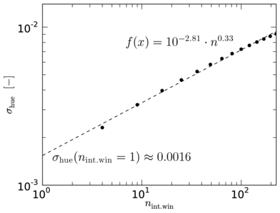
Figure 11. Estimation of the hue error for an interrogation window size of 12 × 12 px using a threshold of 64.
Download figure:
Standard image High-resolution imageUsing again Gaussian error propagation, we obtain  and
and  as maximal values for the absolute and the relative error, respectively. This results in a dynamic range for the actual measurement of (Hmax − Hmin)/σhue ≈ 43.
At this point it should be noted though, that the calibration described above has to be improved in the next steps by incorporating more measurement data, considering the impact of different viewing angles in the same field of view and systematically investigating the use of the evaluation parameters, which influence and can thus be used to optimize bandwidth and the dynamic range.
Other filtering and calibration procedures, as proposed in the literature, e.g. Rao and Zang [32] proposing a 5 × 5 median filter, Grewal et al [33] introducing neural networks and Roesgen and Totaro [34] suggesting a statistical technique using a proper orthogonal decomposition, are promising approaches to further improve the accuracy of the technique.
3. Experimental testing and analysis
3.1. Experimental setup
The investigated mixed convection cell has a square cross section of 500 mm × 500 mm and an aspect ratio between length and height of Γxz = 5 (see figure 12(a)). The air inflow is supplied through a slot below the ceiling, while exhaust is provided by another slot above the floor. Both vents extend over the whole length of the cell. The bottom and ceiling of the cell can be maintained at different temperatures. This setup allows generating mixed convection under well-defined conditions, and serves as a generalized model system for geometrically more complex technical configurations. The flow field and the heat transport within this container have already been presented in some publications: Westhoff et al [35] investigated the low-frequency oscillations of the large-scale circulation, Kühn et al [36] applied a newly developed tomographic PIV technique to large volumes, and Schmeling et al [37] studied the large-scale flow structures and the heat transport using PIV and temperature probes. Again Schmeling et al [38] investigated the large-scale circulations and their oscillations by means of many temperature probes within the cell combined with smoke visualizations.
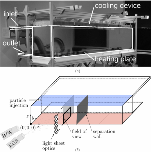
Figure 12. (a): Picture of the mixed convection cell showing the heating plate at the bottom, the cooling plate at the top, as well as the slots for air in- and outflow at the side. (b): Sketch of the experimental setup used for combined PIT and PIV, including the coordinate system and the origin.
Download figure:
Standard image High-resolution imageFor the first experiments with the combined PIT/PIV technique, no external pressure gradient is applied between the inlet and the outlet of the enclosure. Thus, the measurements are conducted rather in pure thermal convection than in mixed convection. Nevertheless, due to the still existing openings of both the inflow and outflow channels, a slow fluid exchange with the surrounding takes place. The fields of view with extensions of approximately 300 × 150 mm2 for PIT and 225 × 150 mm2 for PIV are located close above the heated bottom plate and close to the front side of the enclosure, see figure 12(b) and the coordinate systems in figure 16, where y = 0 and z = 0 is the lower front edge of the enclosure. The difference of the sizes of the fields of view is caused by the different angles under which the cameras are operated. Remapping and superposing the images is realized based on a well-known technique for stereoscopic PIV (e.g. [12]) using recordings of a calibration grid.
The TLC particles are generated with the airbrush system, which is supposed to inject the particles into the settling chamber in front of the inlet for mixed convection cases. During the feasibility tests, as already mentioned, the external volume flow is switched off in order to provide a longer retention period in the cell, therefore, the particles have to be sprayed directly into the enclosure. For illumination of the particles, the specially developed white light sheet based on white LEDs is used. The particle images are recorded with a double shutter grey level and a single shutter colour CCD camera, so that temperatures could be determined from the local hue values and velocities from the local particle image displacements between subsequent recordings. The use of two cameras provides better results than using just a single double shutter colour CCD camera. This is because the less sensitive colour camera can be operated in async. shutter mode, recording only the first of the two light pulses, while the highly sensitive grey level camera is operated in the double shutter mode for the PIV evaluation. Furthermore, the signal to noise ratio of the grey level camera is lower than that of the colour camera, which leads to a higher quality of the PIV results.
3.2. Results I: quality of the results
A raw particle colour image is presented in figure 13(a), to depict the quality and the contrast of the colour images used for the temperature evaluation. A plume of warmer air can already be seen in this picture: the blue part in the centre indicates higher hue values than those of the green and red surroundings. Both frames of the B/W image after high and low pass filtering are shown in figure 13(b). Further, information on the applicability of PIV is given in figure 14, which presents (a) the correlation plane (left) for one interrogation window (24 × 24 px), including the corresponding windows of the two frames (middle and right). The size of the particle images, which is approximately 2 × 2 to 3 × 3 px, the suitable number density of particle images per interrogation window and the clear peak in the correlation plane indicate the high quality of the PIV measurements. Additionally, figure 14(b) reflects the 2D and (c) the 1D pixel displacement distributions; these depict the good quality of the PIV results in terms of the absence of peak locking.

Figure 13. (a) Raw colour image, (b) both frames of the B/W image after high and low pass filtering. Note that the images are unrectified and do not completely overlap. A warmer plume can already be seen in this picture: the blue part in the centre indicates higher hue values than the green: these increased hue values indicate an increased temperature.
Download figure:
Standard image High-resolution image
Figure 14. (a) Left: correlation plane, middle: first image, right: second image. (b) 2D displacement plane and (c) 1D displacement histograms.
Download figure:
Standard image High-resolution imageAfter rectifying, overlapping and evaluating the data, simultaneously recorded instantaneous temperature and velocity fields as depicted in figure 15 can be calculated. The formation of a warm plume which rises from the lower thermal boundary layer can be seen. The top hat of the plume as well as both side vorticities and the root with quickly rising warm air are clearly visible. Such a detailed recorded picture of temperature and velocity of a rising thermal plume has, as far as we know, not been previously recorded experimentally.
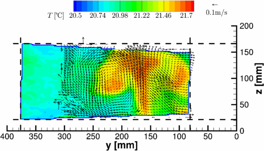
Figure 15. Instantaneous temperature contours and velocity vectors for the above shown raw particle images. For the sake of clarity, only every second vector is shown in each direction. Recorded at Pr = 0.71, Re = 0 and Ra ≈ 9.0 × 10⁷. The colour bar reflects the relative accuracy of σΔT = 0.06 K. The error of the absolute temperatures is σT = 0.19 K.
Download figure:
Standard image High-resolution imageFor the velocity calculation, we use a pulse delay of τ = 16 ms at a light pulse length of 1 ms, which leads to a pixel displacement up to 10 px and therefore a maximal particle shift during one light pulse of less than Δx ≈ 0.7 px. Furthermore, we use an interrogation window size of 24 × 24 px, an overlap of 50%, a three point Gaussian fit for the peak detection, and a seven step multigrid evaluation starting at a window size of 256 × 256 px and disabled sub-pixel image shifting. This results in a vector spacing of approximately 2.5 mm. For the sake of clarity, only every second vector in each direction is shown in figures 15 and 16. The hue values, i.e. the temperature values as well, are calculated using a filter size of 12 × 12 pixel and a threshold of 64, see section 2.4.

Figure 16. Instantaneous temperature contours and velocity vectors for twelve instants in time (Δt = 0.25 s between two images) showing the dynamics within the enclosure. For the sake of clarity, only every second vector is shown in each direction. The legend and the reference vector at the top apply to all images. The colour bar reflects the relative accuracy of σΔT = 0.06 K. The error of the absolute temperatures is σT = 0.19 K.
Download figure:
Standard image High-resolution image
To conclude this subsection, a short discussion of possible errors and limitations resulting from the use of TLC tracer particles, LED based white light illumination, as well as the camera systems will be given. First to be mentioned is the spatial homogeneity of the particle distribution, as in any PIV evaluation. This is already rather good, see e.g. the particle images in figure 13(b). The homogeneity of the illumination is also no problem for this field of view, but might be a more important issue with larger measurement planes due to the divergence of the LEDs. The light sheet thickness, which is approximately 10 mm, is in reasonably good agreement with the interrogation window size used for PIV (≈5 × 5 mm2), but imposes a restriction on the spatial resolution for non-purely 2D flows. These points may cause some errors and limitations, but do not influence the results in our studies negatively so far. Secondly, there are restrictions regarding the maximal flow velocity that can be studied. These are the following behaviour of the tracer particles, which is discussed in detail in section 2.2. The duration of the light pulse limits, in combination with the imaging optics used, the maximal flow velocity as well, because particle images would be smeared out or stretched to stripes for too long pulses in combination with fast flows. In our system, a pulse duration of 1 ms still leads to sharp particle images, see e.g. the particle images in figure 13(b) and 14(a). Thirdly, the accuracy of the temperature and the sensitivity of the hue measurements have been analysed and discussed in section 2.5. Currently, the achievable accuracy in the temperature measurement is limited by the accuracy of the hue temperature calibration, while the hue sensitivity would offer more headroom. Nevertheless, relative temperatures can already be measured with an accuracy of  , which is reflected in the colour bar of the contour plots of our results accordingly.
3.3. Results II: flow analysis
The convective air flow investigated here is induced by a temperature gradient between the bottom and the top plates of ΔT = 7.2 K, while the external pressure gradient is set to zero. This results in the following characteristic numbers: Rayleigh number Ra ≈ 9.0 × 10⁷, Reynolds number based on the inflow velocity Re = 0 and Prandtl number Pr = 0.71. Thus, except for the unsuppressed fluid exchange through the openings of the inlet and the outlet, pure thermal convection is investigated.
The results of simultaneous PIT and PIV measurements in our rectangular convection cell are presented in figure 16, which shows the temperature as contour and velocity, calculated from image pairs by means of well-established PIV algorithms [12], as a vector field. Thereby, the maximal observed velocity is approximately 0.12 m s−1. The images are recorded at a recording frequency of 4 Hz. Figure 16 shows twelve consecutive images, i.e. the time difference between two images is 0.25 s and the series spans a duration of 3 s. A supplemental movie created out of 100 single images at a recording frequency of 4 Hz, i.e. spanning a time period of approximately 100 s is available at stacks.iop.org/MST/25/035302/mmedia.
The parameters used for the PIV and PIT evaluation are the same as described in the previous section, besides the fact that now only every second vector is shown in each direction for the sake of clarity in figure 16 and every third in the movie. Finally it should be noted that no outlier detection is used during the PIV interrogation, but for the visualization, especially in the supplemental movie, a value blanking using a threshold for the velocity is applied to remove distracting vectors.
Figure 16(a) is again the warm plume that was already depicted and described in the section above (figure 15). The time series of images here (a) to (l) shows the breakdown of the typical plume structure towards a thin region of warm rising air at a rather high time resolution of 4 Hz. Thereby, the vortex on the left side of the plume is almost at rest during these 3 s, while the right one convects out of the field of view, leading to the breakdown of the typical mushroom structure. Due to the fact that the velocity and temperature fields are recorded as 2D fields in a plane, it must be taken into account that there will be an out-of-plane component which is not recorded here.
Nevertheless, from the fluid dynamical point of view, the instantaneous temperature and velocity fields recorded at a high frequency open new possibilities in, e.g., analysing the correlation between these two quantities and studying their time evolution. Furthermore, simultaneous measurements will help to further investigate the dynamical processes which lead to, e.g., reorientations and oscillations within convective flows observed, amongst others, in our convection cell [38].
4. Summary and conclusion
We performed combined particle image thermography and particle image velocimetry in convective air flow using thermochromic liquid crystals (TLCs) as tracer particles. The technique allows for simultaneous recording of planar instantaneous temperature and velocity fields. In order to accomplish our measurements, different ways of particle generation were studied and suitable white light sheet optics was developed. The latter generates a white light sheet with a thickness of less than 10 mm over a distance of 500 mm. It is based on light emitting diodes, which guarantee a fast response within less than 50 μs to the trigger signal at rather low cost.
In order to separate the temperature information from the background and pixel noise, a filtering procedure for the recorded colour data was developed. It is based on averaging the hue over interrogation windows while taking into account only those pixels with a V value (HSV) above a certain local threshold. Its working process, applicability and benefits are demonstrated on a synthetic image.
Results from application of the technique to mixed convection in a cuboidal container were presented and discussed. Amongst others, a thermal plume including its mushroom structure, the adjacent vortices and its root with quickly rising warm air could be captured with high spatial resolution. Furthermore, due to a time resolution of 4 Hz, a large fraction of its dynamics could be resolved.
In order to perform quantitative measurements, a fast calibration procedure has been developed and employed which provided a calibration accuracy of the absolute temperatures of σT = 0.19 K in the studied temperature range. By considering the errors of the calibration curve and the hue noise, which has been computed from the measurement data, a standard error for relative temperature measurements as low as σΔT = 0.06 K was calculated, corresponding to a temperature dynamic range based on the investigated temperature interval of 20. The dynamic range on the hue scale, however, is much higher and amounts to 43, revealing an even higher potential of the technique, depending on the accuracy of the hue temperature calibration.
The next steps in further maturing the technique therefore incorporate further research on the hue–temperature calibration in order to push the limits in terms of increased precision as well as the optimization of the measurement and evaluation parameters for higher dynamic ranges for the hue values. Other issues, which have to be addressed to help to establish the technique, are further characterization of TLC particles in air flow. Here we think especially of the colour play, which is known to deviate for dispersed TLC particles from the bulk properties. Knowledge and control of the size dependence of the colour play could help to optimize the measurement and dynamic range in the future. Also, measurements of the exact reaction time of the particles are required to assess the potential of the technique to application in terms of higher velocities.
Acknowledgments
The authors are grateful to Daniel Schiepel for his ideas on the setup of the new lightsheet optics.