

Abstract
A tomographic PIV system composed of 12 cameras has been used to study the object reconstruction accuracy over a wide range of values for the concentration of tracer particles. The relations between particle image density, number of cameras, reconstruction quality, and velocity field accuracy are determined experimentally. The effect of additional cameras is quantified by the reconstruction signal-to-noise ratio and normalized intensity variance. Furthermore, the variation of the reconstruction quality factor with seeding density and number of cameras is estimated considering the 12 cameras case as reference, which has so far only been investigated using numerical simulations.
The accuracy of velocity measurements is investigated by comparing two simultaneous measurements obtained by independent tomographic systems. The measurement error is estimated by the quadratic difference between the velocity measured by the two systems. The importance of the number of cameras and seeding density is investigated. The results yield an optimum source density of 0.5 for a three-camera system and greater than 1.0 for a six-camera system. Doubling the number of cameras returns a broad range for the optimum source density and significantly lower measurement errors.
Export citation and abstract BibTeX RIS
1. Introduction
Tomographic particle image velocimetry (tomo-PIV) has rapidly gained traction as a 3D, 3-C velocimetry measurement technique since its inception by Elsinga et al (2006), in part due to its acute relevance to measurement needs in aerodynamics and turbulence research (see recent reviews, i.e. Scarano, 2013, Westerweel et al 2013). Although tomographic PIV has been shown to be able to operate at relatively high seeding concentration compared to particle tracking methods (0.05 ppp, particles per pixel, Elsinga et al 2006), increasing the latter is always under the scrutiny of the research community in order to perform high-resolution measurements especially to characterize a wide range of scales in turbulent flows. As the density of particle images on the sensors increases, the quality of the tomographic reconstruction decreases due to the interference among particles placed along the same lines-of-sight (see e.g. Elsinga et al 2006). This eventually leads to the formation of ghost particles that contaminate object reconstruction and under some conditions also the cross-correlation signal, in turn biasing the velocity field (Elsinga et al 2011).
A commonly applied metric for quantifying particle density is the ratio between the number of particles and pixels (ppp). By the use of synthetic testing, a limit for an individual camera in a four-camera system was established at approximately 0.05 based on particles of 2.5 pixels mean diameter (Elsinga et al 2006). The ppp does not take into account the particle image diameter and thus provides only a coarse estimate of how 'full' the recordings are with particle images. A parameter for characterizing this effect is the source density Ns introduced by Adrian and Yao (1985) and followed by Novara et al (2010) in the framework of tomographic PIV. The relation between Ns and ppp involves the particle image diameter,

where d τ* is the particle image diameter in pixel units and  is the length of the camera line of sight within the illuminated volume, which is commonly approximated by the volume depth (D). The above relation states that any increase in the particle concentration (ppv), volume depth, or particle image size (e.g. by a larger f-number), will lead to increasing source density.
A range of experiments and synthetic testing has suggested that for the specific case of a four-camera system, the maximum reliable value of Ns is approximately 0.3 (Scarano 2013). The factors leading to this maximum value were already explored by Elsinga et al (2011) and Discetti (2013) where the effect of source density was included in a geometric model to predict the ratio of the number of real particles Np to ghost particles  in a reconstructed volume. Other factors include the number of cameras and the volume depth,
where  is the number of cameras. Note that this equation is valid only for
  < 1. This model predicts that adding cameras to a system allows the source density to be increased without additional ghost particles being formed. However, the applicability of this model for MART reconstruction is tenuous, as equation (2) is only concerned with the number of ghost particles formed, and not their intensity. The iterative nature of the MART procedure is known to shift intensity from the ghost particles to true particles (Elsinga et al 2006). Furthermore, the subsequent cross-correlation analysis is more sensitive to particles of greater intensity. Therefore, equation (2) represents a highly conservative estimate of reconstruction and cross-correlation performance.
As for most experiments, the exact reconstructed field is unknown, and therefore the most practical criterion to assess the accuracy of a tomographic reconstruction is the inspection of the light intensity distribution along the volume depth. The method requires a top-hat-like illumination of the measurement domain. In the illuminated region, both real and ghost particles are formed, whereas outside the reconstructed intensity only ghost particles are formed. This difference in reconstructed intensity allows the reconstruction signal-to-noise ratio (SNRR) to be defined as the ratio of reconstructed intensity of actual particles inside the illuminated region (EI includes actual and ghost particles) and that outside ( includes only ghost particles),
Note that this equation is based on the assumption that the generation of ghost particles is uniform throughout the volume, which is valid for images containing uniform seeding. In contrast to equation (2), the SNRR includes the effect of both the number of ghost particles and their difference in intensity. Several studies are now reported (Elsinga et al 2006, Scarano and Poelma 2009, Fukuchi 2012, among others) which use this metric, where values of 2 or greater indicate an acceptable reconstruction quality, eventually leading to a reliable cross-correlation analysis (Scarano 2013).
The second practical criterion of reconstruction quality considers the normalized variance of the reconstructed intensity within the volume as suggested by Novara and Scarano (2012). A high value of the normalized variance indicates a sparse reconstructed field with high-amplitude peaks. In contrast, a low value is associated with a denser distribution of intensity with lower-amplitude peaks associated with ghost particles. The variance is normalized by the mean value of the volume, yielding the normalized intensity variance 
where i is a voxel index and  is a scalar representing the average intensity of all voxels. The advantage of this metric is that it does not require prior knowledge of the exact object intensity (e.g. in case of non-uniform illumination). Moreover, the reconstruction does not need to encompass the non-illuminated region as required for SNRR. The normalized intensity variance is not as widely reported in literature. Novara and Scarano (2012) proposed that values of
  ranging between 20 and 30 correspond to an acceptable reconstruction quality (Q > 0.7).
A study by Michaelis et al (2010) concentrated primarily on the effect of varying the source density, but they did not consider the use of additional cameras beyond four. Also, the experiments were conducted in water, which posed an early limit to the maximum attainable particle concentration because of medium opacity. A recent effort to realize experiments at increased seeding density was made by Fukuchi (2012) who used a tomographic system composed of eight cameras to reconstruct a thick-volume (approximately 50 mm depth) for studying the wake of a cylinder. A considerable stretch of the operational envelope was obtained, with measurements at a particle image density as high as ppp = 0.5. Experiments were also conducted at ppp of 0.2 and 0.8, showing a dependence of reconstruction signal-to-noise with seeding density. However, the detailed effects of varying the source density were not investigated, for instance by estimating the intensity variance, the reconstruction quality factor, or measurement error.
It is worth mentioning that as an alternative to the approach of adding cameras, an increase of the achievable source density was also explored using motion-tracking enhanced MART (MTE-MART, Novara et al 2010), which takes into account simultaneously the two exposures for the particle field reconstruction. Its application to turbulent shear flows (Novara and Scarano 2012) showed that a seeding density up to 0.2 ppp can be treated by a four-camera system. However, the MTE-MART technique involves computational efforts an order of magnitude greater than standard tomographic PIV, making it suitable only in specialized circumstances. Other recent works include the spatial filtering improved tomographic PIV approach by Discetti et al (2013), which uses a tailored filtering of the reconstructed volume between MART iterations to reduce ghost particle intensity, and the simulacrum matching-based reconstruction enhancement (SMRE) technique proposed by de Silva et al (2013), which aims to remove ghost particles a posterori the reconstruction process. The latter reported notable improvements in reconstruction quality for source densities up to around NS=0.4. Another recent approach by Elsinga (2013) uses particle-tracking velocimetry (PTV) to identify ghost particles in time-resolved sequences and remove them from the reconstructions. A similar approach but integrated with an iterative particle reconstruction technique (IPR; Wieneke 2013) is the 'shake-the-box' approach of Schanz et al (2013).
The above studies underline the relevance of obtaining a tomographic system able to deal with high seeding density. Despite these efforts, there is no conclusive statement on the relations between particle tracers concentration, their density in the recordings, the number of cameras and the final accuracy of reconstruction as well as that of the velocity field. In particular, the simultaneous variation of seeding density and cameras over a wide and controlled range has not been investigated experimentally, which is explored in the present work. The results are compared with available data from literature obtained from synthetic tomographic PIV data and by the theoretical model of performance given by equation (2).
A tomographic system composed of 12 cameras is realized to enable the investigation. Experiments are conducted in the wake of a circular cylinder immersed in a low-speed wind tunnel, with the particle concentration slowly varying throughout the experiment. A method is devised for an accurate determination of the concentration, based on a dual-volume-thickness simultaneous measurement described in section 2.4. The reconstruction quality is examined in section 3 following three criteria: the reconstruction signal-to-noise ratio, normalized intensity variance, and the quality factor Q* from a system containing fewer cameras to one containing the full set of 12 cameras. The accuracy of the velocity measurements is estimated considering the disparity between the instantaneous velocity fields obtained from independent tomographic systems, in section 4.
2. Experimental apparatus and procedure
2.1. Flow facility and measurement conditions
The experiment is performed in an open-circuit, open-test-section tunnel with test cross section of 40 × 40 cm2 (W-tunnel) at the Aerodynamics Laboratories of TU Delft Aerospace Engineering. A cylinder of 6 mm diameter spans the entire height of the test section and generates an unsteady wake, characterized by large-scale spanwise-coherent vortex shedding. The arrangement is schematically shown in figure 1. The tunnel is operated at an exit velocity of 12 m s‒1, corresponding to a Reynolds number of 5000 based on cylinder diameter.
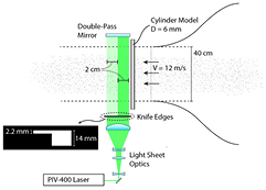
Figure 1. Schematic of experimental setup with details of illumination system and the stepwise varied knife-edge filter.
Download figure:
Standard image High-resolution image2.2. Tomographic system
A stage-smoke generator produces water-glycol droplets of approximately 1 micron diameter. To vary the particle seeding throughout the experiment, the laboratory is first filled to a high concentration of seeding particles. At the start of the experiment, an exhaust fan gradually vents the room, lowering the particle concentration.
The measurement volume size is 4 cm along the cylinder span, and 14 mm in depth. The volume is illuminated by a double-cavity Spectra-Physics Quanta-Ray PIV-400 Nd:YAG laser (400 mJ pulse‒1). Light sheet optics shapes the 6 mm diameter beam into a collimated beam of rectangular cross section propagating parallel to the cylinder axis. An additional 90-degree high-power laser mirror is used to double-pass the laser slab through the measurement volume, which homogenizes the intensity across the cameras used in forward and backward scattering configuration. The time separation between laser pulses was set to 40 µs, yielding average displacements of approximately 0.5 mm (12 pixels) in the free stream region.
The illuminated volume has different thickness in two regions: close to the cylinder the thickness is 14 mm to measure the entire wake produced by the cylinder. Downstream, the thickness is reduced to 2.2 mm to enable an accurate estimate of the tracer's concentration. This configuration is realized by a knife-edge filter as illustrated in figure 1.
The 12-camera tomographic system is organized in a cross configuration to maximize the total angular aperture of the system (approximately 40 degrees total angle in both horizontal and vertical direction) as shown in figure 2. Twelve LaVision Imager LX 2MP interline CCD (1628 × 1236 pixels, pixel pitch 4.4 µm) are used, equipped with 75 mm focal length objectives attached to custom-manufactured Scheimpflug adapters. The aperture is set to f/# = 8. The corresponding diffraction image size of particles is dτ = 11 μm. Spatial autocorrelation analysis yields a particle image diameter of 2.05 px. The estimated depth of field is 18 mm, ensuring in-focus particle images through the entire depth of the measurement volume.
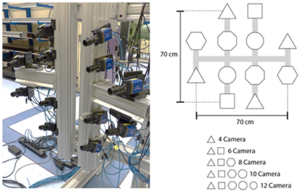
Figure 2. The 12-cameras tomographic imaging system (left) and schematic description of cameras selection for the tomographic sub-systems (right).
Download figure:
Standard image High-resolution imageA summary of illumination and imaging parameters is given in table 1.
Table 1. Summary of physical parameters of the experimental setup.
| Parameter | |
|---|---|
| Pixel size | 4.4 µm |
| Sensor size | 1628 × 1236 |
| Magnification | 0.10 |
| Digital resolution | 23.8 px/mm |
| Objective focal length | 75 mm |
| F-number | 8 |
| Particle image diameter | 2.05 px |
| Laser pulse separation | 40 µs |
| Laser energy | 400 mJ/pulse |
The cameras are connected to a host computer equipped with three Gigabit Ethernet boards, and controlled using LaVision Davis 8.1 software and a PTU9 timing unit. Tomographic calibration is performed using a dual-plane target (LaVision Type 7). Initial fitting errors were in the range of 0.3 pixels. The volume self-calibration technique (Wieneke 2008) using a set of 50 images at low seeding density (ppp < 0.02) corrects the mapping function to within 0.01 pixel for all cameras. The self-calibration procedure was performed before and after each measurement as calibration errors are known to severely affect the reconstruction accuracy (Elsinga et al 2006).
2.3. Data processing
Image pre-processing consists of two steps: first, the historical minimum is calculated at each pixel for each camera. Then the images are subtracted by the corresponding minimum. This has been suggested by Fukuchi (2012) as a method better suited for high source densities compared to local kernel methods such as sliding minimum subtraction. Following this, noisy fluctuations of the background intensity were estimated to be approximately 60 counts. This constant value was subtracted from the images. No spatial filtering (smoothing) or intensity normalization is applied. A sample preprocessed image for a value of NS approximately 0.7 is shown in figure 3. Note the change in density across the image, corresponding to the knife-edge transition from 14 to 2.2 mm thickness.

Figure 3. Sample image (cropped along height) after image preprocessing. Corresponds to a central camera of the cross configuration.
Download figure:
Standard image High-resolution imageAll measurements are performed simultaneously with the 12 cameras and subsequent operations consider subsets as illustrated in figure 2. The selection of cameras composing each subset maximizes the angular total of each subsystem.
The reconstruction is conducted using the fast MART algorithm within the LaVision 8.1 software, which corresponds to a more efficient implementation of the sequential MART algorithm, i.e. Elsinga et al (2006). The computations are optimized taking into account the sparsity of the reconstructed volume and voxels with intensity below a specified threshold level are not updated (Atkinson and Soria 2009). The threshold level of 0.001 counts was determined by comparison to the conventional MART algorithm taken for reference. The settings for the processing are outlined in table 2. The reconstruction volume depth is increased by approximately 25% in the front and rear to be able to estimate the SNRR. The reconstructed volume size is thus 47 × 52 × 19 mm. The calculations were performed on a 24-processor PC and the reconstruction time was approximately 5 min for a four-camera system and 15 min for the 12 cameras system.
Table 2. Summary of reconstruction parameters.
| Parameter | |
|---|---|
| Reconstruction algorithm | MART |
| Volume size [px] | 1118 × 1237 × 452 |
| Volume size [mm] | 47 × 52 × 19 |
| Digital resolution | 23.8 vox/mm |
| Reconstruction tterations | 8 (7 with smoothing) |
| Diffusion coefficient | 1.0 |
| Initial value | Uniform (value 1.0) |
| Relaxation parameter | 1.0 |
2.4. Particle concentration
The particle density varies in time throughout the run. At the beginning of the experiment, the highest concentration of particle tracers is approx. 40 part mm‒3 (as determined by the following analysis). The concentration decays by venting the room during the experiment. As a result, a continuous range of particle concentrations is experienced; however, an in-situ method is required for an accurate determination of the concentration, ppp, and source density at each snapshot. In a tomographic PIV experiment, the particle image density on the cameras is typically too high for an unbiased estimate based on 2D peak detection. As the particle image density exceeds approximately 0.04 ppp (Fukuchi, 2012), the number of detected particles no longer follows a linear relationship with the number of true particles due to high overlap probability. From previous studies dealing with this problem, the most practiced technique for concentration measurement is the slit-test (e.g. Novara and Scarano 2012, Schanz et al 2013, Fukuchi 2012, among others). A removable slit acts as knife-edge filter placed into the laser beam before it reaches the laser volume. The reduced thickness of the laser illumination results in a lower particle image density, allowing an accurate estimate of particle concentration by 2D peak detection. The actual particle image density is estimated by multiplying the obtained particle density by the ratio of the slit to full volume thickness.
This technique can be applied provided that two caveats are considered. First, the method requires the seeding density to be held constant during the time between the recordings with and without the slit. Second, because of differences in optical magnification and viewing angle, the seeding density varies from camera to camera. The present approach addresses both issues. First, the experiment is designed such that the slit measurement is simultaneous to the thick volume measurement (figure 3), which enables a particle density measurement while the concentration is varying in time.
Because the volumetric particle density (ppv, particles per voxel) does not vary depending on the viewing angle like the particle image density, the former is considered for estimating the particles' concentration. Tracer particles are counted by a 3D peak-finding algorithm within the reconstructed volume corresponding to the slit region, where the 12-camera system is essentially free from the phenomenon of the ghost particles. This was further verified using fewer cameras, and the estimated ppv did not change when at least 6 cameras were used.
The 3D peak-finder operates on a 6-connected neighborhood, which is considered to be a robust approach in view of the sparsity of the reconstructed object. The corresponding ppp is obtained by multiplying the ppv by the volume thickness and it represents the particle image density that would be detected by a camera with a viewing axis normal to the illuminated volume median plane.
The time history of measured C, ppv, ppp, and NS within the experiment are given in figure 4. At the beginning of the experiment, the particle concentration exceeds 40 particles mm‒3, which corresponds to a source density of approximately 3.5. During a period of 300 s, the seeding density decays to values reported in many tomographic PIV experiments for air flows (Scarano 2013), with particle concentration around 3–5 particles mm‒3 and a source density of 0.25–0.5. The scatter in particle concentration is largely due to small inhomogenetities in the seeding of the room, leading to slightly higher or lower concentration. This was verified by inspection of the particle images that exhibited the same trend as figure 4.
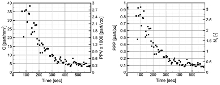
Figure 4. Volumetric particle concentration/particles per voxel (left), particle image density (particles per pixel) and source density NS (right). (Values of ppp and NS refer to the region of full illumination.)
Download figure:
Standard image High-resolution image3. Reconstruction quality
3.1. Reconstruction signal-to-noise ratio
As reported in previous studies, the most prominent artifact of MART reconstruction for a particle field is the presence of ghost particles. In the illuminated region, both real particles and ghost particles are formed, whereas outside the reconstructed intensity only ghost particles are expected to form.
As more cameras are added, fewer ghost particles are formed with the double effect of increasing the signal level within the laser sheet and decreasing it outside. Figure 5 illustrates a reconstructed intensity profile along the volume depth making use of 4, 6, and 12 cameras. The data is taken from an average of five snapshots at approximately NS = 1.4. The intensity is normalized by the maximum of each profile. As more cameras are added, the intensity outside of the laser sheet is dramatically reduced. The average value inside and outside the laser sheet is estimated by the solid and dashed lines, and represents EO and EI in equation (3), respectively. The reconstruction signal-to-noise ratio SNRR is reported in figure 5. The four-camera system yields SNRR < 2, while for 12 cameras SNRR approaches 5.

Figure 5. Tomographic reconstruction intensity profiles and SNRR values for 4 (left), 6 (center), and 12 (right) cameras. Results obtained with source density Ns = 1.4.
Download figure:
Standard image High-resolution imageExtending the procedure to the entire experiment transient yields the relation between the SNRR and the source density for different numbers of cameras. Results are plotted in figure 6. Note that the condition SNRR > 2 is met at a source density up to 0.9 for the four-camera system, 1.9 for six cameras, and beyond 3.0 for the 12-camera system. As a result, one may conclude that experiments conducted with more than six cameras satisfy the reconstruction quality criterion even at particle image density up to 0.5 ppp, which significantly moves forward the value currently practiced (ppp = 0.05, Elsinga et al 2006) by about one order of magnitude. The latter result agrees with the experimental observations made by Fukuchi (2012).

Figure 6. Reconstruction SNR for varying numbers of cameras and varying source density.
Download figure:
Standard image High-resolution image3.2. Normalized intensity variance
The same procedure is followed to generate the normalized intensity variance (equation (4)). Only the regions of the reconstruction within the illuminated volume are considered. Figure 7 (left) shows the value of  The trend is consistent with that of SNRR, with higher values obtained at low particle concentration indicating a high signal sparsity and low occurrence of ghost particles. The variance of the reconstructed object increases when more cameras are added. However, the difference in variance between systems of different numbers of cameras is not as pronounced as for the SNRR. For example, if a criterion for acceptable reconstruction quality is taken with a variance above 20, then the improvement in source density moving from four to six cameras is only of 0.6, compared to 1.0 suggested by the SNRR criterion.

Figure 7. The normalized intensity variance σE*as a function of the source density and number of cameras.
Download figure:
Standard image High-resolution imageThe value of the variance shown in figure 7 is comparable to the results shown by Novara and Scarano (2012), who reported typical values of the variance for converged MART with different cameras and the application of MTE in the range of 20–30. The maximum reported value of  for a four-camera system in their work is approximately 28, which compares well to the four-camera system operating at a source density of 0.9 in the present study. In conclusion, the agreement suggests a design note for tomographic PIV reconstructions: the normalized intensity variance should exceed 20 to compare with reconstruction SNR beyond 2 and ensure a reliable analysis by cross-correlation.
3.3. Relative quality factor
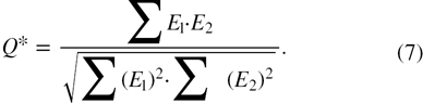
The use of a relatively large number of cameras enables the evaluation of reconstruction accuracy by the quality factor Q. The latter is defined as the normalized correlation coefficient between the reconstructed volume and the exact intensity distribution (Elsinga et al 2006). In contrast to the SNRR and  which are properties of a reconstructed object, the quality factor specifies the degree of matching to a reference reconstructed object and is therefore a more rigorous check of the reconstruction quality. This criterion has been modified by Novara et al (2010) for experimental data, considering the normalized cross-correlation between the reconstructed object E1 and a reference object E2,
Note that the mean value of E1 and E2 are subtracted. E1 and E2 are chosen such that E1 is a reconstruction with a smaller number of cameras (i.e. E1 = ENc=4) and E2 is a reconstruction with the full number of cameras (E2 = ENc=12). These values are denoted as Q* and shown in figure 8.
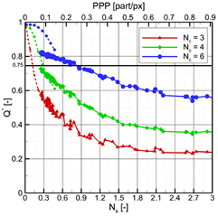
Figure 8. The quality factor Q*. Dashed lines in the Q* figure indicate values from numerical simulations given in Scarano (2013).
Download figure:
Standard image High-resolution imageA solid horizontal line provides the reconstruction quality criterion (Q > 0.75) proposed by Elsinga et al (2006) on the basis of numerical simulations. Furthermore, part of the diagrams obtained with synthetic data in Scarano (2013) are shown as overlays. At low seeding density (NS < 0.3), only the four- and six-camera systems are able to achieve reconstructions with a quality factor around 0.75. The reduction of Q* is significant as the number of cameras is reduced. For the systems with fewer cameras, the downward trend in reconstruction quality comes back to an agreement with available data from Scarano (2013) until approximately NS of 0.4.
A discrepancy is noted between the data from the six-camera system and synthetic data, attributed to the use of the 12-camera data as the reference volume. Because the 12 camera system also contains reconstruction artifacts, the value of Q* will not asymptote to a value of 1.0. However, a clear trend can be noted in the data, which allows a connection to be made between the quality factor and the reconstruction SNR. For Q*, the 0.75 threshold is crossed at an NS of 0.9 and 0.3, respectively. The corresponding SNRR for these cameras at this source density is 4.5 and 5, respectively.
4. Analysis of velocity fields
4.1. Procedure and processing
Although the seeding concentration varies throughout the experiment, the analysis of the velocity field measurement is performed maintaining constant the size of the interrogation box to 32 × 32 × 32 voxels. The overlap factor is kept at 75%. With a particle concentration of 5 particles mm‒3 (average concentration from 400 to 600 s), the number of particles inside the window is approximately NI = 24, ensuring a robust analysis by cross-correlation.
An in-house algorithm (Fluere) performs 3D cross-correlation by the multi-pass, multi-grid volume deformation (VOLDIM) method similar to that used in Scarano and Poelma (2009). Correlation is performed using symmetric block direct correlation and Gaussian window weighting. Spurious vectors are detected by universal outlier detection (Westerweel and Scarano 2005) and replaced with a distance-weighted neighborhood average. No spatial filtering (smoothing) is applied to the final vector field.
4.2. Instantaneous snapshots
A visual inspection of the measured velocity field by means of Q-criterion visualization (Hunt et al 1988) of vortices is given in figure 9. The conditions are taken as the same shown earlier for the reconstruction (NS = 1.2, NC = 3, 6, and 12). The calculation of the velocity gradient tensor components is based on second-order central finite differences.

Figure 9. Velocity fields for three-camera (top), six-camera (center), and 12-camera (bottom) reconstruction. Isosurfaces given for positive values of the Q-criterion, color-coded by volume depth.
Download figure:
Standard image High-resolution imageThe largest flow features are the spanwise coherent rollers, which are captured in all cases. At the present Reynolds number (Re = 5000), the turbulent regime results in significantly smaller flow scales compared to, e.g., Scarano and Poelma (2009). Although the general topology of vortices is still reproduced at such a high seeding density for the three-camera system, the secondary rollers mostly inclined along the streamwise direction are not captured especially by the three-camera system, whereas they become visible in the snapshot reconstructed by 12 cameras. Elsinga et al (2011) found that the flow topology remains unaffected by increased levels of ghost particles. However, a gradient modulation effect is visible for the three-camera analysis, with the large-scale coherent structures along the span of the model diminished in intensity and appearing intermittently broken apart.
4.3. Error analysis
A quantitative comparison is not straightforward since the actual velocity field is unknown. A method is followed here that directly estimates the velocity error by comparing the measurements from two independent systems. Under the assumption that the error from such two systems is uncorrelated, the error estimate is taken as the norm of the difference between the two velocity fields. Additionally, the objects composing the pair considered for cross-correlation are taken by different sets of cameras. This is done in order to minimize any possible correlation/bias from ghost particles. For example, to calculate the first displacement (viz. velocity) field  frame 1 from system 1 would be correlated with frame 2 from system 2. The opposite is used to calculate
  The error
  is computed as the average norm of the difference of these fields following Christensen and Adrian (2002),
In the above equation, i is the index of each gridpoint, and N the total number of vectors in the measurement domain. This approach not only accounts for the random error, but it also considers the effect of calibration errors. Although useful in the present case where two tomographic PIV systems are used, the present method is generally not viable for studies where a single tomographic system is used. Therefore, the results are also compared with the error estimator based on the velocity divergence operator. For an incompressible flow, any nonzero measured value of the divergence is ascribed to measurement errors. This error  has been related to the standard deviation of the measured divergence via linear error propagation, under the assumption that the errors at neighboring grid points are uncorrelated (Atkinson et al 2011),
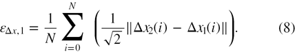
In the preceding expression,  is the standard deviation of the divergence field and h is the grid spacing (8 voxels presently). Figure 10 presents the
  (left) and
  (right) for three-, four-, and six-camera systems. At relatively low source density (NS < 0.5) the measurement error is dominated by the limited number of particles within a window in the cross-correlation analysis. In particular, the values of
  at low seeding density is little dependent upon the number of cameras used. As the particle density is increased, both
  and
and  decrease, which is ascribed to the higher number of particles considered for the cross-correlation. Further increases of seeding density show a greater disparity between the systems of different numbers of cameras. This indicates that the error here becomes dominated by the reconstruction accuracy, which prevails over the increase of cross-correlation accuracy and robustness.
Figure 10. Velocity error magnitude  (left) as a function of the source density for 3, 4, and 6 camera cases. On the right plot, the standard deviation of velocity divergence is shown on the right axis and the corresponding error estimate
  according to equation (9).
Download figure:
Standard image High-resolution image
The minimum error for both estimators ( and
and  ) results from a minimization of the combined effect of limited particles within the interrogation volumes and reconstruction artifacts. In the three-camera system, a minimum error is
  approximately 0.6 vox at a source density NS = 0.5. In comparison, the six-camera system attains a minimum error
  of approximately 0.35 vox across a broad range of source densities ranging from NS = 1.0–2.5.
It is worth noting the discrepancy between  and
and  in general, the values of
  are found to underestimate
  by approximately 30%, which is ascribed to the fact that for the grid points used for the finite differences estimate of the divergence, the random error is not uncorrelated. Moreover, any error arising from discrepancies in the geometrical calibration of the two separate tomographic systems will not be accounted for by the divergence estimator.
The error magnitude reported here is comparable to numerous studies in the literature. In Scarano and Poelma (2009), a cylinder wake at Reynolds number of 1000 was investigated using a four-camera system, with a standard deviation in the divergence of 0.02. This is lower than the values in figure 10, which is ascribed to the greater spatial resolution and lower Reynolds number of the experiment. Atkinson et al (2011) performed an experiment in a turbulent boundary layer with discrete volume offset methods and reported a divergence of 0.05, which corresponded to a velocity error of 0.5 px; these values compare favorably with the four-camera case. Wieneke and Taylor (2006) reported errors of around 0.2 vox for a laminar flow with low velocity gradients. This wide variability in reported error estimates is in part due to the variation in complexity of the underlying flow field. It is well established that the different flow regimes and properties of the turbulent flow can cause large discrepancies in the measured random error.
In conclusion, the trends shown in figure 10 provide guidance for choosing the optimal source density that maximizes the accuracy of the velocity estimation for a given number of cameras.
5. Conclusions
The effect of seeding density and number of cameras on tomographic reconstruction quality and velocity measurements has been studied experimentally. Measurements were performed varying the particle density in a controlled manner. A 12-camera system provides the baseline to make highly accurate reconstructions that are considered for reference when evaluating the accuracy of reconstruction from subsystems.
The objects reconstruction accuracy was analyzed using three metrics: reconstruction SNR, normalized intensity variance, and relative quality factor based on various camera configurations. Each metric indicated an increase of system performance as additional cameras were added: based on an SNR threshold of 2, a four-camera system was able to perform successful reconstructions at a maximum source density of approximately 0.9, and a six-camera system increases this to approximately 1.9.
The normalized intensity variance was found to observe a similar, but not identical trend as the reconstruction SNR. A value of 20 is suggested as a threshold for successful reconstructions, confirming previous results from Novara and Scarano (2012). The authors encourage the use of this criterion as a complementary tool to the reconstruction SNR.
The relative quality factor Q* is given as a more rigorous estimate of the reconstruction quality. It shows a more constrained view of performance compared to the reconstruction SNR and normalized intensity variance. For achieving the Q = 0.75 criterion from Elsinga et al (2006), the limiting values of NS for a four-camera and six-camera system are 0.3 and 0.9, respectively.
The velocity field was compared across a range of source densities and with various camera configurations. A qualitative overview yields a similar large-scale flow topology, relatively unaffected by changes in the number of cameras. Instead, small-scale features and structures coherent over the span of the model showed distortions when reconstructed by fewer cameras. A quantitative analysis of the error level was obtained by evaluating the velocity disparity between independent measurement systems and invoking the continuity equation (divergence-free velocity field). The measurement error reaches a minimum, indicating an optimum value for the source density, given the camera configuration. Tomographic systems composed of small numbers of cameras reach this optimum for lower values of NS (NS = 0.5 for NC = 3). A six-camera configuration appears to approximately halve the error and the range of optimum operation is broader (1.0 < NS < 3.0).
Acknowledgments
This research is supported by the European Community's Seventh Framework Programme (FP7/2007–2013) under the AFDAR project (Advanced Flow Diagnostics for Aeronautical Research). Grant agreement No. 265695.