

Abstract
A new equation for the convective heat loss from the sensor of a hot-wire probe is derived which accounts for both the potential and the viscous parts of the flow past the prongs. The convective heat loss from the sensor is related to the far-field velocity by an expression containing a term representing the potential flow around the prongs, and a term representing their viscous effect. This latter term is absent in the response equations available in the literature but is essential in representing some features of the observed response of miniature hot-wire probes. The response equation contains only four parameters but it can reproduce, with great accuracy, the behaviour of commonly used single-wire probes. The response equation simplifies the calibration the angular response of rotated slanted hot-wire probes: only standard King's law parameters and a Reynolds-dependent drag coefficient need to be determined.
Export citation and abstract BibTeX RIS

Original content from this work may be used under the terms of the Creative Commons Attribution 3.0 licence. Any further distribution of this work must maintain attribution to the author(s) and the title of the work, journal citation and DOI.
1. Introduction
A hot-wire probe, in its simplest form, consists of a thin sensing element supported by two prongs attached to a stem. The probe operates by exposing the sensing element to a fluid stream and measuring the rate of convective heat loss  . The heat loss is related to the flow velocity and direction by a calibration law. A calibration law which accurately models the response of the probe is an indispensable ingredient of flow measurements with hot-wire probes. For a heated wire with length-to-diameter ratio greater than 200, exposed to a stream of speed u and direction orthogonal to its axis, King [1] suggested that

where  is the total loss rate,
  the heat loss rate in absence of flow and B a constant coefficient. Equation (1) has underpinned most of the anemometry work to this day. Collis and Williams [2] later showed that a better representation for the heat loss rate is

with  . A similar value is normally found when calibrating commercially available hot-wire probes.
In flows with far-field velocity at an angle β to the direction orthogonal to the sensor (see figure 1), King's law (1) implies
where q is usually referred to as the effective cooling velocity and β the yaw angle. Shubauer and Klebanoff [4] reported data fitting equation (3), but only for  .
.
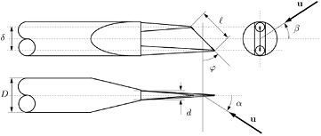
Figure 1. The main dimensions of a slanted hot-wire wire probe and the pitch (α), yaw (β) and slant angles (φ).
Download figure:
Standard image High-resolution imageEquation (3) represents the simplest embodiment of the directional sensitivity of a hot-wire probe. King [1] also observed that the angular response of these probes could be used to determine the flow direction as well as the magnitude of the flow velocity. Skanstrad [3] devised a slanted wire probe, exploiting this directional sensitivity, to measure Reynolds stresses in turbulent boundary layers. Data from probes of various characteristics, however, show significant departures from the behavior described by equation (3) and a large body of literature has been generated over the years in an attempt to relate the effective cooling velocity to the flow velocity far away from the probe.
Newman and Leary [5] found that the angular response of hot wires is approximated more closely by

with  at low Mach numbers. Sandborn and Laurence [6] performed measurements over a wire range of yaw angles β and Mach numbers and found that the cosine law (3) only represented measured data correctly at very low Mach numbers. Furthermore, to match data at
  , i.e. with flows nearly parallel to the sensor, they proposed—albeit with reservations—a relation containing terms associated to the component of the flow tangential to the wire:

Hinze [7] also proposed an equation for the effective cooling velocity containing a small contributions from the velocity component tangential to the sensor:

with κ in the range 0.1 and 0.3 and with values increasing with decreasing velocitiy. In a similar vein, but writing a decade later, Jørgensen [8] proposed an expression for the squared effective cooling velocity based on the velocity components in the wire frame of reference vi:

but his data showed that the  coefficients are in reality sensitive to the probe orientation. Webster [9] analysed the response of probes with sensor length-to-diameter ratios
  but for a limited range of speeds and found that the yaw response could be reasonably well represented by Hinze's expression (6) with
  . Champagne et al [10] performed detailed measurements of the temperature field of hot-wire probes and concluded that the heat loss rate is indeed sensititve to the velocity component tangential to the wire. They found that equation (6) could represent heat transfer data from wires with length-to-diameter ratios above 200 with
  for
for  , with κ decreasing to essentially 0 for
  . Champagne's experiments were carried out with wires of identical diameters and their results on the sensitivity of κ on the ratio
  may well be interpreted in terms of prong distance-to-diameter ratio. The findings in Champagne et al were then used by Champagne and Sleicher [11] to derive a response equation which took into account tangential velocity components as well as large turbulent fluctuations.
Friehe and Schwartz [12] proposed a modified cosine law

In this expression, b is a parameter sensitive only to the sensor length-to-diameter ratio. b is insensitive to velocity and yaw angle, at least for  . Based on their modified cosine law, Friehe and Schwartz showed that the κ parameter in (6) must also be a function of yaw angle and showed that Champage's data [10] support this conclusion.
Bruun [13] reviewed some aspects of hot-wire calibration and recommended a response law of the type

and reported measurements showing the variation of the response with flow velocity, pitch (see figure 1) and yaw. However, in discussing some practical aspects of hot-wire calibration, Bruun [14] later recommended a response function similar to the one proposed by Newman and Leary [5].
In reality, the angular response of hot-wire probes is inextricably linked to the relation between the velocity in the stream far away from the probe and the velocity near the probe. This relation is determined by the aerodynamic interference of the structures supporting the sensor. Champagne et al [10] suggested that the angular response of slant wires probes deviates from the cosine law because of the presence of a tangential velocity component induced by the asymmetry of the prongs.
Comte-Bellot et al [15] systematically studied the effect of interference from the prongs and from the stem. The overall effect of the interference from the components of the probe is to decrease the effective cooling velocity with respect to the free stream when the wire is aligned with the flow, and to increase it when the wire is orthogonal to it. Furthermore, it was found that the perturbation induced by the prongs has a dominant effect on the response of the wire, and that it is inversely proportional to the prong spacing δ. This scaling is consistent with potential theory [16] and will be used—in a slightly modified form—in this paper. Strohl [17] studied the effect of interference on Reynolds stress measurements with rotated hot-wires and showed that aerodynamic intereference by the elements supporting the sensor can alter the measured values by up to 16% for commercial probes.
Brehmorst [18] also studied the aerodynamic intereference of the prongs on the wire and suggested that the apparent variation in κ with pitch could be attributed to the flow being channeled between the prongs. Adrian et al [19] used the slender body approximation to the potential flow of the prongs and the stem to study the aerodynamic interference between the supporting elements and the sensor, and estimated its effect on the yaw and pitch response by estimating the velocity perturbations induced at the midpoint of the sensor. The comparison was based on original data as well as Comte-Bellot's data and found that the effect of each element could be superimposed seperately. Bruun and Tropea [20] performed measurements of the response of probes with single normal, and slanted wires and found that the coefficients in Jørgensen's equation, as well as the linear coefficient in King's law, change with pitch.
Fujita and Kovasznay [21] presented a rotated slanted wire technique for the simultaneous determination of three normal and one Reynolds shear stress. The technique was based on a least squares fit of a number of measurements taken with a single probe, exposed to the flow at several angles. The technique used the response equation

valid for yaw angles above  . The quantity
  in equation (10) is an empirical parameter and varies with the mean velocity. Kuroumaru [22] measured three velocities and six Reynolds stresses with a slanted hot-wire behind a fan impeller. Their measurement technique relied on finding the minimum response orientation to determine the flow direction and then on a least squares procedure to determine the remaining properties of the flow. In view of the difficulty of fitting trigonometric expressions to the measured response to pitch variations, their response law was based on a polynomial representation for the sensitivity to pitch, and a trigonometric expression for the sensitivity to yaw. Samet and Einav [23] noticed that the sensitivity to yaw angle β depends on pitch angle α. In particular, they noticed that at
  the response is monotonic, but not at higher yaw, therefore precluding the possibility of finding velocity from a regression technique.
Buresti and Di Cocco [24] combined Jørgensen's equation and a coordinate transformation to show that the effective cooling velocity is a bilinear function of the velocity vector of the type

where aij depend on the orientation of the probe and on its slant angle. Buresti and Di Cocco, however, did not discuss the implications of aerodynamic interference on their method. The bilinear form of Buresti and Di Cocco's response equation results in algebraic relationships between the time-mean and the mean-square fluctuating response of the sensor and the velocities and Reynolds stresses. The validity of the relations was demonstrated through numerical tests. Wagner and Kent [25] also used Jørgensen's equation on rotated straight wires and found that using coefficients determined at selected flow directions yields sufficiently accurate velocities. Russ [26] presented a set of response equations based on Jørgensen's equation, King's law and a coordinate transformation together with a least-squares procedure to determine velocities and Reynolds stresses for a nearly one dimensional flow. The method used the assumption of low-turbulence intensity and one-directional mean flow to obtain a simplified form of the response equations presented in Buresti and Di Cocco [24]. The coefficients were determined from calibration data.
Peña and Arts [27] presented a slanted hot-wire method for the measurement of three velocity components and six Reynolds stresses. The method relied on Jørgensen's equation and a response equation based on coordinate transformation. The method was tested in a wall jet flow with favourable results when compared with PIV data. The calibration curves for Peña and Arts' probe show the peak response at  pitch located at
  . Such response would be produced by Fujita and Kovasznay's [21] response equation but not from the other equations reported earlier in this section. Stella et al [28] presented a generalised form of Jørgensen's equation in tensor form which allowed the calibration of hot-wire sensors with respect to pitch as well as yaw response. Whilst reporting the relation between effective cooling velocity and sensor orientation, Stella et al pointed out that the components of the tensor appearing in the response equation ought to be determined via calibration, rather than evaluated from the geometric parameters of the probe.
This brief review shows that a large number of response equations, summarised in table 1, have been proposed over the years. Some of these relations are, however, only valid over a narrow range of yaw and pitch angles. The most recent slanted wire methods rely on modified forms of Jørgensen's equation and King's law and assume a bilinear relation between wire response and velocity. However, no attempt has been reported so far to derive a response equation incorporating directly the potential and viscous effects of the prongs and the stem on the velocity in close proximity to the sensor. The purpose of this paper is to derive such a response equation and to demonstrate its validity for commonly used probes. The view will be taken that the convective heat loss rate can be determined in two conceptual steps. In the first step the velocity in proximity of the wire is related to the velocity far upststream of the probe when mounted in a calibration facility or, equivalently, to the velocity at the position of the sensor if the probe was removed from the flow. In the second step the rate of heat loss from the sensor is related to the velocity in its proximity.
Table 1. Summary of angular response equations. Only equations (5) and (10) can produce maximum effective cooling velocity at  .
.
 |
Year, authors | Remarks | |
|---|---|---|---|
| (3) |  |
1946, Shubauer and Klebanoff [4] | From King's law,  , low Mach. , low Mach. |
| (4) |  |
1950, Newman and Leary [5] | Low Mach. |
| (5) |  |
1955, Sandborn and Laurence [6] | Wide β-range. |
 |
|||
| (6) |  |
1959, Hinze [7] |  , ,  . . |
| (8) |  |
1968, Friehe and Schwartz [12] |  . . |
| (10) |  |
1968, Fujita and Kovasznay [21] |  . . |
| (7) |  |
1971, Jørgensen [8] | Velocities in wire-fixed frame. |
| (9) |  |
1971, Bruun [13] | |
| (11) |  |
1987, Buresti and Di Cocco [24], | |
| 1997, Stella et al [28] | Tensor aij from calibration data. |
2. Experimental apparatus
The data presented in this paper were measured in a small open loop tunnel with vertical flow axis. Ambient air is drawn in through a thick gauze and a honey-comb screen into a 4:1 contraction nozzle discharging into a cylindrical test section. The nozzle diameter is  mm. The test section has diameter of
  and length
  .
.
The turbulence intensity in the potential core of the jet is found to be less than 0.1%. The exit of the test section features an additional thick honeycomb section. The facility is drawn down by a constant speed fan and the flow rate is regulated via a throttling valve at the exit of the flow path.
At the beginning of each set of measurements, the facility is run for 30 min to allow the temperature and pressure in the laboratory to settle to a steady state. A settling time of 1 s is also allowed before measurements are taken after the probe is moved to its new position during angular traverses.
The velocity of the potential core of the jet is recorded indepenently of the hot-wire probe via a dual head pitot probe located near the hot-wire sensor. The pitot probe heads have diameter of approximately 10d, d being the diameter of the prongs of the hot-wire probe (see figure 1) and are placed at a distance of approximately 100d from the hot-wire sensor during normal operation. The pitot readings are recorded manually using a micromanometer. The hot-wire probes are inserted from the side of the facility through a harness which allows pitch and yaw variations. The mechanism is powered by two stepper motors.
The hot-wire probes are operated in constant temperature mode with oveheat ratio 1.8. The dead voltage is determined by recording the signal from the hot-wire probe with the facility switched off and with a lid placed on the entrance and at the exit throttling valve completely closed to prevent spurious circulation of air. The dead voltage is measured at the beginning and at the end of the test. Data are acquired through a standard anemometer. The acquisition time at each measuring point is 20 s at a sampling rate 100 kHz.
3. Methodology
In order to build a response model for a conventional slant wire probe, the prongs are idealised as two semi-infinite bodies of revolution of identical shape and diameter D, but offset in length with respect to the x12 plane by a distance  , δ being the distance between the axis of the two prongs and φ the slant angle (see figures 1 and 2). The tips of the prongs are represented as truncated cones, but any shape can be catered for.
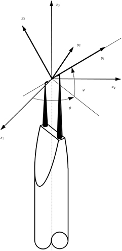
Figure 2. Hot-wire probe frames of reference. The frame  is the laboratory frame of reference. The frame
  is the probe frame of reference. The probe has slant angle φ. The plane π containing the prongs and the sensor forms an angle θ with the
  plane.
Download figure:
Standard image High-resolution imageThe wire is idealised as a straight line segment between the points  and
and  , located on the tips of the short and long prongs, respectively. A coordinate ξ is introduced on the wire, its value being 0 at
  and 1 at
  . The length of the wire is
  and is approximately equal to
  . The effect of the wire on the flow pattern is neglected throughout this paper.
A wire frame of reference is introduced, with the  axis aligned with the wire and oriented from the short prong to the long prong, the
  axis normal to the plane containing the prongs and
  completing a right-handed orthogonal system, as shown in figure 2. At a probe angle
  , the probe rests with its prongs in the
  plane and its axis parallel to the x3 axis. A velocity vector
  in the laboratory frame of reference and its representation
  in the wire frame of reference are related by the linear transformation

where the matrices  and
and  are
are
The velocity at a location  along the wire differs from the velocity in the far-field on account of the potential field of the prongs and their wakes. This difference is also equal to the difference between the measured velocity and the velocity at the location of the sensor if the probe was removed from the flow.
The potential part of the flow around the prongs can be represented by a dipole distribution  ,
,  being a pair of coordinates specifying the position of any point on the surfaces of the prongs. The corresponding velocity field is [16]
In equation (14),  is the surface of the two prongs,
  is the normal to the prongs surface and
  is the distance vector between any point
  and a point on the prongs surface

For a given far-field velocity  , the dipole distribution is the solution of the problem
where  is any generally integrable function defined on the surface of the prongs. This problem can be solved numerically using standard techniques [29]. It is convenient to represent the flow field of the prongs as the superposition of three distinct fields, each corresponding to the solution of the problem (16) with unperturbed velocity of unit magnitue, aligned with one of the coordinate axis and with the prongs in the x13 plane:
where  is the prong diameter-to-spacing ratio. This induces the same scaling with prong spacing as found by Comte-Bellot et al [15]. The non vanishing components of the tensor
  are shown in figure 3 for two probes with different values of ε. It can be seen that the ε-scaling holds with very good approximation near the mid-point of the sensor, i.e.
  . It can also be seen that the largest interference effects are to be expected at the ends of the sensor. For arbirtrary probe angles θ the velocity field induced in the proximity of the wire is a linear function of the velocity vector at a large distance from the probe


Figure 3. The contribution of the potential flow around the prongs to the perturbation velocity in the proximity of the wire from equation (18).  ,
,  :
:  ;
;  , •:
, •:  ;
;  ,
,  :
:  ;
;  ,
, :
:  ;
;  ,
,  :
:  . Empty symbols for
  , filled symbols for
  .
.
Download figure:
Standard image High-resolution imageThe velocity in proximity of the wire, expressed in wire coordinates, is therefore
The tensor Lij is a function of the probe orientation and slant angle. The tensor  is a function of the position along the wire, of the geometry of the probe as well as probe orientation.
The displacement effect of the boundary layers and wakes being shed from the prongs can be approximated by using the method of surface sources [30], as customarily done when coupling boundary layer calculations with inviscid calculations. For the purpose of the present analysis, it is sufficient to use a uniform surface source strength, related to the magnitude of the far-field velocity through a coefficient Cd. In general, Cd depends on the Reynolds number. For the sake of simplicity it will be assumed that Cd is constant in the range of velocities for which the probe has been calibrated. This is the case for Reynolds numbers based on flow velocity and prong diameter between 20 and 80. For a dipole distribution  and in absence of oncoming flow, the velocity induced in the space surrounding the prongs is
The velocity induced by the boundary layers and wakes is given by the solution to the problem
so that the velocity induced at the sensor, in the wire frame of reference, is

The non-vanishing components of  are shown in figure 4 for
  and
and  , where it can be seen that the interference from prongs wakes and boundary layers also scales with .

Figure 4. The contributions of Cd to the perturbation velocity in proximity of the wire from equation (20).  ,
,  :
:  ;
;  , •:
, •:  . Empty symbols for
  , filled symbols for
  .
.
Download figure:
Standard image High-resolution imageIt is now possible to write the velocity at the sensor in terms of the far-field velocity and of the interference effects due to the potential and viscous flow field of the prongs:

The convective heat flux can be obtained from the velocity in equation (23) by integrating along the wire a cooling law of the type (6)
where the tensor Jhk is

and  represents distribution of difference between the flow temperature and the wire temperature as well as the effect of additional coatings on the surface of the wire. For sensors with plated ends, the effect of the coating is to remove the contribution to the integral in equation (24) from the parts of the sensor where the disturbances generated by the prongs are largest. The coefficient κ is retained in the formal derivations, but its value is set to zero in the rest of the paper. Champagne results [10] show this to be the correct value for a sensor in isolation, i.e. for
  .
.
The external product  can be written in terms of far-field velocity components
where


The convective heat flux can finally be written in terms of the far-field velocity and interference effects:
with


Equation (33) is the sought for response model for a slanted wire probe, including an approximation to the viscous behaviour of the prongs. For practical computations, the integral in equation (33) cannot be evaluated analytically, but can be evaluated using numerical integration rules. In the following, 8-point Gauss-Lobatto formulae have been used.
Equation (33) can be also approximated by a Taylor series in ε around  to find
where
Equation (36) shows that the complex behaviour described by equation (33) reduces to an effective cooling velocity which is a bilinear function of the far-field velocity for probes with very widely spaced prongs, i.e.  . For probes of finite spacing, the heat loss rate contains a correction proportional to ε and is made of two contributions. The first contribution is also a bilinear function of the far-field velocity and is due primarily to the potential flow of the prongs. The second contribution is linear with respect to the the direction of the velocity vector, but quadratic in its magnitude, and is due to the wakes and the boundary layers of the prongs.
For a far-field velocity aligned with the wire, the response equations (33) and (36) predict heat loss from the sensor even if  . This is due to a small velocity with direction orthogonal to the wire induced by aerodynamic interference by the prongs. Therefore, even if a local cooling law which is not sensitive to longitudinal velocities is used, an overall response similar to Hinze's [7] and Jørgensen's [8] is predicted. The apparent values of the longitudinal sensitivity coefficients, κ in equation (6) and
  in equation (7), would however be sensitive to the flow direction, as indeed found in experiments.
4. Results
One of the most visibile consequences of the interference from the prongs and the stem on response of a slanted sensor is that the maximum response at  pitch does not take place at
  . Furthermore, at pitch angles diffent from
  , the maximum response takes place at a probe angle generally dependent on the pitch. This causes the apparent dependence of Hinze's and Jørgensen's coefficients on flow direction, as recorded by some researchers in the past. Data clearly showing such behaviour were published by Peña and Arts [27].
This phenomenon can be studied by tracing the amplitude of the response  and the probe angle
  at which it occurs as the displacement coefficient Cd and the pitch angle α are varied. This study can be performed computing the variation of the solutions of the equation
as α and Cd are varied. The study is performed for both models (33) and (36) with reference to slanted wire probes of prong diameter-to-distance ratios  and
and  . The results of the study are shown in figures 5 and 6, respectively. In the absence of viscous effects, i.e.
  , the response predicted by both equations (33) and (36) is symmetric with respect to the plane containing the prongs. This places the maximum response of the probe at
  . This shows that the viscous contribution from the flow around the prongs is a main factor in the shape of the response of hot-wire probes. The boundary layers and wakes of the prongs make the flow asymmetric with respect to the plane containing the sensor, thereby moving the maximum response away from
  at
at  pitch by as much as
  , as seen in the insets in figures 5 and 6.

Figure 5. The maximum response of a slanted wire probe with varying pitch angle α and displacement coefficient Cd. Probe with  . Solid lines: model in equation (33), dashed lines: model in equation (36).
  .
.
Download figure:
Standard image High-resolution image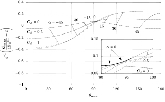
Figure 6. The maximum response of a slanted wire probe with varying pitch angle α and displacement coefficient Cd. Probe with  . Solid lines: model in equation (33), dashed lines: model in equation (36).
  .
.
Download figure:
Standard image High-resolution imageAerodynamic interference also changes the amplitude of the maximum response, on account of velocity components orthogonal to the sensor associated with the flow pattern between the prongs. The response functions proposed by Fujita and Kovasznay [21] can reproduce this feature of the response, at least at  pitch. The results in figures 5 and 6 also show that the maximum response moves further away from
  the higher Cd at a given pitch angle α. Furthermore, probes with more widely spaced prongs exhibit smaller deviation from symmetry and the linear/bilinear response in equation (36) provides a good approximation for their behaviour. Probes with closer prongs show a higer sensitivity to the pitch and larger deviations from a linear/bilinear response. In practical terms, this means that probes with more widely spaced prongs can be better represented by simpler calibration laws based on equation (6) or (7).
The response of four real probes is compared with the response predicted by equations (33) and (36) in figures 8–11. The probes used in this study are shown in figure 7. The data in figures 8 and 9 refer to straight wire probes, figures 10 and 11 refer to slanted wire probes, The comparison is performed at yaw angles between  and
and  and pitch angles
  and
and  and at Reynolds numbers based on prong diameter
  between 10 and 30. For all probes the response is modeled using
  and
and  and only the coefficients of B and n are modified. The prong diameter-to-spacing ratio is approximately
  for the proebs b and d, and approximately
  for the proebs a and c.

Figure 7. The four probes used in this study. a: DANTEC 55P11, b: DANTEC 55P01, c: DANTEC 55P12, d: DANTEC 55P02.
Download figure:
Standard image High-resolution image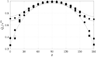
Figure 8. Angular response of probe a:  ,
,  (straight wire probe).
  ,
,  , B = 0.45, n = 0.44. Solid lines: equation (33), dashed lines: (36).
  :
:  ,
,  :
:  ,
,  :
:  . Empty symbols:
  , half-filled symbols:
  , filled symbols:
  .
.
Download figure:
Standard image High-resolution image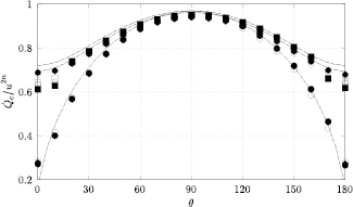
Figure 9. Angular response of probe b:  ,
,  (straight wire probe).
  ,
,  , B = 0.45, n = 0.44. Solid lines: equation (33), dashed lines: (36).
  :
:  ,
,  :
:  ,
,  :
:  . Empty symbols:
  , half-filled symbols:
  , filled symbols:
  .
.
Download figure:
Standard image High-resolution image
Figure 10. Angular response of probe c:  ,
,  (slanted wire probe).
  ,
,  , B = 0.45, n = 0.44. Solid lines: equation (33), dashed lines: (36).
  :
:  ,
,  :
:  ,
,  :
:  . Empty symbols:
  , half-filled symbols:
  , filled symbols:
  .
.
Download figure:
Standard image High-resolution image
Figure 11. Angular response of probel d: slanted probe  ,
,  (slanted wire probe).
  ,
,  , B = 0.45, n = 0.44. Solid lines: equation (33), dashed lines: (36).
  :
:  ,
,  :
:  ,
,  :
:  . Empty symbols:
  , half-filled symbols:
  , filled symbols:
  .
.
Download figure:
Standard image High-resolution image
The graphs show the ability of the response equations (33) and (36) to reproduce the behaviour of real probes with only four parameters, κ, Cd, B and n, of which only B and n are optimised for each probe. The value of Cd is likely to change at Reynolds numbers outside the range explored in the present study.
The response of straight wire probes is found to be symmetric with respect to the probe orientation: the maximum response is found at  independently of α. This shows that for straight probes the effect of interference on the angular response of the sensor can be hidden in the calibration coefficients of a simple cooling law.
The response of slanted wire probes is more complex and exhibits a response sensitive to the pitch angle. Both the response at  yaw and the yaw angle at which the maximum response take place depend on the pitch angle. Both responses are represented correctly by the proposed laws, except at yaw angles in the range
  –
– , where the short prong and the sensor are immersed in the wake of the long prong.
Lastly, some final observations are in order regarding the computational cost of the proposed response equations. The evaluation of the effective cooling velocity for a given probe orientation using the expressions in Buresti and Di Cocco [24] and Stella et al [28] require one three-by-three matrix-vector product and one scalar product. The evaluation of the effective cooling velocity via equation (36) requires two three-by-three matrix-vector products and two scalar products. Finally, equation (33) requires M matrix-vector products and 2M scalar products if M Gauss-Lobatto integration points are used. Considerations of computational cost become important when processing large amounts of data obtained, as an example, by traversing in a plane or when computing flow statisticis in statistically non-stationary flows.
5. Conclusions
An accurate representation of the probe angular response is an essental ingredient of measurements taken with rotated slanted wires. The relationship between the response and the flow direction is complicated by the flow field around the prongs supporting the sensor, which alters the direction and magnitude of the velocity in the proximity of the sensor with respect to the direction and magnitude of the far-field velocity. A large number of response equations have been proposed over the years in an attempt to describe the sensitivity of slant wire probes to yaw and pitch angle. These relations are not satisfactory in that they are valid over a limited range of yaw angles and cannot reproduce the correct value of the angle of maximum response  . As a result, the calibration of hot-wire probes for rotated slanted wire anemometry has to rely on the acquisition of a large amounts of data for curve fitting.
A new directional response model for slanted wire probes has been presented here which is based on a detailed description of the flow around the prongs of the probe. For the first time in literature, quantitative and detailed estimates of both the inviscid and viscous contributions of the prongs to the flow field around the probe are given. The model also accounts for the variability of wire temperature and flow conditions along the wire. The proposed model is embodied, in its most general form, by equation (33). The model characterises the behaviour of hot wire probes using only four adjustable parameters, namely the King's law parameters B and n, Hinze's parameter κ and a displacement coefficient Cd.
The general response equation (33) can be approximated by a Taylor series in the prong diameter-to-spacing ratio ε. The resulting approximate response law (36) is very accurate even for miniature probes but is more easily handled than the full model for the purpose of data processing.
Equation (36) is marginally more expensive than those proposed by Buresti and Di Cocco [24] and Stella et al [28] but is more accurate and instructive, whilst being far easier to handle than the full response equation (33).
From a practical point of view, the findings in this paper allow the directional response of slanted wire probes to be reduced to the determination of the standard King's law parameters B and n and a displacement coefficient Cd. These quantities can be accessed with far fewer measurements than those required for a traditional full directional response calibration.
Acknowledgments
The authors gratefully acknowledge Rolls-Royce plc and the UK TSB TuFT programme for funding this work and granting permission for its publication. The authors wish to thank Prof N A Cumpsty and Dr J S S Wong for their comments and suggestions during the preparation of the manuscript.