Abstract
Among the main vibration-to-electricity conversion systems, resonant harvesters suffer from a series of strong limits like their narrow frequency response and poor output power at small scale. Most of all, realistic vibration sources are variable in time and abundant at relatively low frequencies. Nonlinear vibration harvesters, on the other hand, are more attractive, thanks to their large bandwidth response and flexibility to convert kinetic energy of the natural frequency of the sources. In particular, bistable oscillators have been proven to show higher global performances when excited by random vibrations. In this paper, such an approach is investigated for piezoelectric beams by exerting an increasing axial compression. An advantage of this technique is the absence of magnetic forces to create bistable dynamics. A thin piezoelectric axially loaded beam is theoretically modelled and experimentally investigated under wideband random vibrations. In the buckled configuration, the device exhibits superior power generation over a large interval of resistive load, with gains up to more than a factor of ten compared to the unbuckled state. The numerical model and experimental results are in good qualitative agreement.
Export citation and abstract BibTeX RIS
1. Introduction
The conversion of dispersed energy in the environment into usable electrical energy has been revealed to now be a realistic alternative for the powering of small devices, thanks to the recent advances in ultra-low-power electronics. Among various renewable forms of energy, mechanical vibrations are deemed to be one of the most attractive power sources for low-power electronics owing to its power density, versatility and abundance in real environments. Vibration-to-electricity conversion via piezoelectric materials has been investigated by many researchers [1–4]. They provide high output voltages and have compact size. Furthermore, piezoelectric devices do not need an external voltage source and can be adapted for micro-electromechanical systems (MEMS). On the other hand, traditional vibration energy harvesters are based on linear resonators which have the inherent limitation of operating at their resonant frequency in order to maximize the output power. The increase in the mechanical damping represents the easiest method to widen the frequency response, but with the drawback of reducing the maximum power. Furthermore, as dimensions shrink below a few millimetres, resonance rises over the kilohertz region. Thus, MEMS-sized linear harvesters are very inefficient in the real world, where the kinetic energy is often located below a few hundred hertz with variable intensity and wide bandwidth [5–8]. A smart energy harvester should feature a high response over a large frequency interval, self-tuning features and be capable of adapting to variable acceleration levels. Some research groups have explored the approach of oscillator arrays in order to cover a large frequency range by overlapping their responses [9–11]. Although this method widens the frequency spectrum, the overall power per unit of volume is decreased. In order to overcome the problem of resonance tuning, particularly for small oscillators, Leland and Wright [12] proposed a tunable-resonance piezoelectric vibration energy harvester (VEH) by applying an axial compression so as to lower its resonance frequency. Other research groups have employed a frequency up-conversion technique [13, 14]. This method can be implemented in different ways, for example by using mechanical frequency rectification or particular magnetic coupling. However, there are still problems of coupling loss and frequency dependence. In order to improve the versatility and adaptation to different applications and environments, an increasing interest is being recently oriented to the exploitation of more complex nonlinear systems. In this regard, Jung et al [15] have presented an interesting energy harvester that uses resonating cantilever beams attached to buckled slender bridges. The piezoelectric cantilevers are excited when the buckled bridges snap through two equilibrium positions, so making them resonate at their natural frequency even if the input excitation is off-resonance. A prior nonlinear electromagnetic harvesting generator was proposed by Burrow and Clare [16] for vibration energy harvesting. Then, the employment of piezoelectric nonlinear Duffing oscillators for energy harvesting has been investigated by the authors of this work [17, 18]. In these works the bistability was implemented by adding opposing permanent magnets to a piezoelectric cantilever beam. Subsequently, other research groups verified that bistable harvesters show enhanced performance when excited by periodic excitation [19, 20] or under wide bandwidth vibrations away from the resonant frequency [21]. Enhanced oscillations are produced with respect to the linear configuration when the acceleration intensity is high enough to make the inertial tip mass jump between two stable positions. As a consequence, in a bistable configuration, the oscillator follows higher energy orbits. The electrical power dissipated into a resistive load is amplified by more than a factor of four compared to a linear arrangement and reaches a maximum for a particular potential barrier height depending on both the distance between the magnets and the intensity of input vibrations. The exploitation of a Duffing oscillator for energy harvesting was also discussed in [18] and tested by Erturk and Inmann [22]. They have experimentally verified an order of magnitude larger performance of a non-resonant piezomagnetoelastic cantilever against a linear resonant configuration. Enhanced bandwidth response has also been demonstrated by Stanton et al [23] through the use of softening and hardening effects within the quadratic potential field of a piezoelectric beam with permanent magnets. Most of the Duffing-like generators so far discussed have been implemented by adding permanent magnets. However, in several applications of wireless sensor networks, magnetic fields could strongly interact with the electronics of the sensor nodes. Moreover, at micro- and nanoscales it is very difficult to integrate permanent magnets within the generator. Therefore, a bistable energy harvester without the addition of a magnetic field would be more desirable. A theoretical analysis of piezoelectric buckled beams was previously made by Maurini et al [24] and Giannopoulos et al [25]. However, this research was mainly focused on static actuation operational mode, without envisaging random vibrations. Bistable snap-action microsystems were also studied by Casals-Terré et al [26] but not involving piezoelectric materials.
In this work we investigate the electrodynamical response of the piezoelectric buckled beam operating as a kinetic-to-electrical energy converter. The buckling structure is used to implement a bistable magnetic-free vibration energy harvester. Theoretical and experimental studies are here presented to compare the output response of a linear versus nonlinear dynamical regime of such a piezoelectric clamped–clamped beam.
2. Theoretical framework
2.1. Analysis of the model
The energy harvesting system that we consider is based on a piezoelectric beam clamped on both ends on a base excited vertically by a shaker. One of the two clamps is fixed, while the other can be moved through a micrometric stage.
Figure 1 shows a diagram of the piezoelectric buckled bridge. In our case, it consists of a support of a thin steel beam with one or two bonded layers of piezoelectric material of width b. These are assumed to be polarized only along the z axis. An additional inertial mass can be arranged on the centre of the bridge in order to vary the dynamical response of the system. Two electrodes are placed on both surfaces of the beam and collect the current which then flows into a resistive load. The clamping support is assumed to vibrate only vertically. The total beam deflection is equal to w(x,t). As a first approximation, the main contribution to the electrical field along this direction is due to the electromechanical coupling related to the horizontal strain of the beam. Therefore, the constitutive equations for the piezoelectric effect are as follows [27]:
where Tx and Sx represent mechanical stress and strain, Ez and Dz are respectively the electric field component and electric displacement along the z axis,  is the elastic stiffness of the piezoceramic layer at constant electric field, and ezx and
  are the piezoelectric coupling constant and electric permittivity at zero strain. The structure is initially compressed by moving one end towards the other so as to fit in the distance L. By gradually changing the compression distance ΔL we explore the system electrodynamics from the monostable to the bistable regime.

Figure 1. (a) Schematic diagram of piezoelectric buckled bridge. (b) Section of the steel support and piezoelectric layer (bimorph). (c) Equivalent electrical circuit of the harvesting system.
Download figure:
Standard imageThe analytical model of the system is derived from the first-order composite plate theory according to Reddy [28]. The piezoelectric beam is supposed to be homogeneous with constant moment of inertia and stiffness over the whole structure. In order to derive the motion equations of the transverse deflection, we will first proceed to calculate the Lagrangian functional. When the clamping base oscillates with amplitude y with respect to the ground, the total kinetic energy of the beam is the sum of the energy of the steel shim and that related to n piezoelectric layers:
A symmetrical bimorph piezoelectric beam is assumed for simplicity with Lp = L, whereas w(x,t) is the mid-plane deflection along the z axis, and ρs and ρp represent the steel shim and piezoelectric material density with sectional area, respectively equal to As and Ap. Actually, in the experimental device the piezoelectric layer is not continuous along the x axis. A small gap is left in the middle of the beam in order to have room for an additional mass M0 to be added. The last term accounts for its kinetic energy. A comprehensive treatment of this case was made in [29]. Moreover, the electrodes are connected in parallel only at one of the two sides of the beam, with length Le < L. Therefore, in the following, we will not consider a self-cancelling electromechanical coupling coefficient. The strain along the x axis, associated with the mid-plane displacement field (u,w), respectively along the x and z axes, is calculated using von Kàrmàn nonlinear relations [28]:
where the first term of the strain is related to the axial in-plane forces and the second term is the curvature due to the bending moment. Since the electromechanical coupling is present, the total potential energy of the composite laminate includes the bending energy, the work done against the induced electric field and the work done by the external compressive forces. Consequently, the total potential energy is expressed as

where V is the entire domain of the composite beam and W is the work done by the external compressive force P applied at the movable tip which is given by

where w' stands for a derivation with respect to x. The last integral above is nonzero only in the post-buckling case. The compressive load is always taken as larger than the critical load so that P > Pcr in order to realize the buckling. db represents the contraction length from side wall pressure corresponding to the critical load Pcr. Manipulation of equation (4) is simplified by introducing the following relations:
where Q(k) is the first element of the in-plane kth layer stress-reduced stiffness matrix, which corresponds for isotropic material to the Young's modulus. Np and Mp are respectively the in-plane force and bending moment due to the piezoelectric coupling. The position of the kth layer is indicated by zk. By substituting equations (1) and relations (3) in (4) and using (6) yields
The terms containing B vanish in the case of a symmetric laminate, as is supposed here. Note that stress-stiffening effects result from external compressive forces and residual piezoelectric stress  . For slender beams, the longitudinal motion can also be neglected compared to the transversal one. As a result
  can be approximated as follows:

Evaluating expressions (6), considering two piezoelectric layers, gives


where Is and Ip are the second moment of inertia of the steel shim and piezoelectric layers, while the electric field is expressed in terms of a time derivative of the flux linkage as  in case active layers are connected in series. The Lagrangian functional of the buckled piezoelectric beam results in

Before proceeding with the calculus of the Euler–Lagrange governing equations, it is worth making some assumptions on the trial functions of vibration mode shapes. We are interested in the dynamic response of the system around the first buckling mode, which is supposed to be dominant. The total deflection with respect to the clamping base can be defined as

where w1 = h0φ1(x) is the initial equilibrium shape of the beam and h0 = w(L/2,0) being the height of the central point at t = 0, whereas v(x,t) is the time-dependent deflection around the initial shape. According to the Galerkin discretization, v(x,t) can be expanded into a superposition of N orthonormal basis functions φi(x) as
where ri(t) are the time-dependent expansion coefficients of the modal configurations. Hence, by replacing (12) in equation (11) and keeping only the first mode, the total deflection results in

where r1(t) is the time-dependent displacement of the middle point of the clamped–clamped beam around the initial buckled shape. Discontinuity of the piezoelectric beam can be treated by using stepwise functions with the continuity and compatibility conditions at the boundaries of each uniform beam section. The boundary conditions of a clamped–clamped beam are w(0,t) = 0, w(L,0) = 0, ∂w(0,t)/∂x = 0 and ∂w(L,t)/∂x = 0 and mode shape functions are taken from prior works [28, 30, 31].
In the following, only the first mode will be considered. Therefore, injecting (13) into the Lagrangian functional (10) gives
where the superscript dot denotes the time derivative and the sixth term is rewritten in terms of equivalent capacitance  of the piezoelectric beam, qhile m, η, k0, k1, k2 and k3 are the effective mass, inertia force factor, piezoelectric coupling factor, in-plane piezoelectric force factor, linear and nonlinear stiffness of the beam, respectively. These parameters are evaluated as follows:


in which the time-dependent first mode is expressed as (h0 + r1(t))φ1 = q(t)ψ, where the initial buckling shape function results in ψ(x) = (1 − cos(2πx/L))/2.
At this stage, single-degree-of-freedom motion equations for vertical deflection of the beam midpoint can be evaluated by applying Euler–Lagrange equations to (14):
where F(t) and I(t) respectively represent the generalized force and current within the energy harvesting circuit. Equivalently, the current will be related to effective electrical load RL by Ohm's law  . Hence, computing (16) gives two second-order nonlinear differential equations that link the motion of the midpoint to the output voltage across the resistive load:

The viscous damping is accounted for by the second term in the first equation. Here, it can be noted that time-dependent variables are not completely separated. In the case k1 was zero, the equations reduce to those of the nonlinear piezoelectric cantilever seen in [22, 17, 19]. In addition, the conservative force is a Duffing-like type, but the linear stiffness parameter is a function of the output voltage. As a continuous piezoelectric layer is assumed over the whole length of the beam, the stiffness parameter k0 should vanish. However, in our experimental model, the electrodes which capture the charge are of length Le < L and are connected only from one side of the beam. Thus, the parameters k0 and k1 are evaluated from zero to Le. Accordingly, all the coefficients (15) are then calculated as


In this paper, our intent is to solve the dynamical equations with stochastic base excitation for an increasing contraction length ΔL. For this purpose, the compression load P, which is unknown in the experiment, can be expressed in terms of ΔL, using the following relationships:


and, in turn, ΔL can be expressed as initial midpoint height h0 and buckling displacement db. This relation is obviously valid only for the post-buckling situation. The critical load for such a clamped–clamped beam is retrieved by Reddy [28]. In the following sections we will make use of numerical methods to solve the motion equations in the post-buckling configuration (17) in order to compare them with experimental results.
2.2. Potential energy analysis
In this section, we consider the case of an analytical system similar to the experimental device, in order to investigate the main dynamical behaviour under random noise excitation. However, for the real system, some corrections to geometrical parameters will be taken into account, as described in section 3. Table 1 summarizes the main model parameters used for simulations and experiments. As a first instance, we can consider the situation at open circuit. Thus, the effective potential relative to the midpoint vertical coordinate q reduces to a quartic function given by

When the beam is compressed by increasing ΔL or, equivalently, the lateral load P, the stiffness parameter k2 becomes negative. As a consequence, the potential energy varies from being a nearly flatted parabola to a double-well function. So that, as expected, the systems behaves as a Duffing oscillator for k2 ≥ 0, which corresponds to a small compression (P ≤ Pcr) or even a tension P < 0, and as a Duffing bistable oscillator for k2 < 0 (P > Pcr). Clearly, a supercritical bifurcation occurs when P − Pcr (or equivalently k2) changes sign, as can be seen in figure 2.
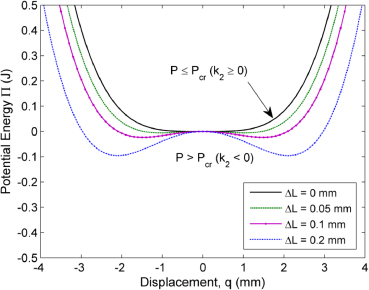
Figure 2. Elastic potential energy of the beam for increasing values of the compressive load corresponding to Δ = 0, 0.05, 0.1 and 0.2 mm.
Download figure:
Standard imageTable 1. Model parameters used for numerical and experimental tests.
| Steel shim | Piezoelectric layer | ||
|---|---|---|---|
| Parameter, symbol | Value | Parameter, symbol | Value |
| Material | Steel | Material | PZT film |
| Length, L0 | 55 mm | Length of layers, Lp | 55 mm |
| Width, b | 11 mm | Length of electrodes, Le | 21 mm |
| Thickness, hs | 0.1 mm | Width, bp = b | 10 mm |
| Density, ρs | 7850 kg m−3 | Thickness, hp | 0.08 mm |
| Young's modulus, Es | 2.03 × 10¹¹ Pa | Density, ρp | 4000 kg m−3 |
| Damping ratio, ζ | 0.018 (unb) | Young's modulus, Ep | 4 × 10¹⁰ Pa |
| 0.025 (buck ΔL/L = 0.4%) | Coupling coefficient, d31 | −10 pC N−1 | |
Electrical permittivity, 
|
100ε0 | ||
| Vacuum permittivity, ε0 | 8.854 × 10⁻¹² F m−1 | ||
For k2 ≥ 0, the potential has an absolute minimum at q = 0 around which the system oscillates with a natural frequency  in the undamped case. Whereas, for k2 < 0, the quartic potential has two local minima corresponding to stability positions q− =− (|k2|/k3)−1/2 and q+ = (|k2|/k3)−1/2. The barrier height hb between the two wells is equivalent to
  . Depending on it and on the vibration noise strength, the system tends to oscillate around either minima and, from time to time, it jumps across the barrier following Kramer's transition rate [32].
Actually, in the dynamical regime, the stiffness coefficient k2 depends on the output voltage. Therefore, the potential energy varies in time. Moreover, in the real experiment, the beam has only one piezoelectric layer, which means that the term B in expression equation (7) is nonzero, so making the potential energy asymmetrical. Such an asymmetry, though, can be considered as not important for a qualitative comparison of the power performance.
3. Experimental and numerical validation
This section deals with the experimental investigation of the real system dynamics together with its global power performance. The theoretical model described above is numerically simulated and taken as a reference for qualitative comparisons. Motion equations (17) are numerically integrated by means of the Euler–Maruyama method, with design parameters listed in table 1, using Matlab® software.
For practical reasons, only the fundamental vibration mode of the beam is considered, because it is supposed to be dominant. The displacement of the central point of the testing beam is measured under random exponentially correlated noise. For both experimental and numerical simulations, different sample functions of the random signal were used for each time series. These measurements were performed by setting various initial compressive lengths, in order to investigate different nonlinear dynamics and stress-stiffening effects. The output voltage is also studied by varying the resistive load and the average power calculated.
3.1. Experimental set-up
The equipment used for experimental tests is shown in figure 3(a). The piezoelectric beam is clamped on both its ends as shown in figure 3(b). One of the two clamps is kept fixed, while the other one was manually moved by a micrometric stage with spatial resolution of 0.01 mm. The piezoelectric sample was manufactured by Ferrari's research group at the University of Brescia (Italy) by screen-printing low-curing-temperature lead zirconate titanate (PZT) films on steel lamina. The main geometric and electrical properties are listed in table 1. However, some differences in the real sample with respect to the numerical model must be specified. The experimental device is made of a steel shim upon which four piezoelectric layers are printed using a PZT milled powder (Piezokeramica APC-856) and low temperature polymeric vehicle-binder mixed in a ratio of 2:1 wt. They are polarized in opposing directions under a 4 MV m−1 electric field perpendicular to the lamina. The total piezoelectric film thickness is 0.08 mm. Hence, the testing system results in a unimorph asymmetrical beam. Measured electrical permittivity and density, after the printing process, are respectively equal to  (±10) and ρp = 4000 kg m−3. The piezoelectric film is also discontinuous in the middle, where a 10 mm gap is depleted to leave room for an additional mass. Thus, the actual length of each piezoelectric strip is 21 mm. The effective capacitance of each piezoelectric side was measured with an RLC meter resulting in around Cp = 1.15 ± 0.05 nF, in very good agreement with the calculated value of 1.16 nF. Two electrodes were screen-printed and fired at low temperature using a conductive silver-based polymeric ink. Electrical contacts are clamped on only one side of the bridge connecting a variable resistance (ranging from 10 Ω to 1 MΩ). Two laser displacement sensors (Keyence LK-501) are used in differential mode to detect the position of the beam midpoint relative to the vibrating base. An accelerometer (PCB Piezotronics 338A35) is also used in determining the base acceleration level in order to minimize inaccuracies. Input vibrations are generated by using a signal generator (Agilent 33220A) and a National Instruments DAQ USB card connected to the power amplifier of the electromagnetic shaker (TIRA). In addition, the input vibration spectrum is monitored by a 1 GHz oscilloscope (Le Croy LC574A). The voltage drop across the resistance together with all other measured signals are captured by a computer through a NI DAQ card with sampling frequency of 2 kHz.
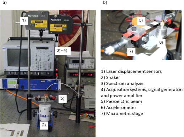
Figure 3. (a) Experimental set-up for system testing. (b) Close-up view of the piezoelectric bridge.
Download figure:
Standard imageIn the experimental system, a small mass of 1.47 g was added at the centre of the beam in order to improve dynamic flexibility. For the theoretical model, this variation implies an additional lumped mass to be included in the kinetic energy term. However, deviations from the theoretical model were expected due to the asymmetry of the structure, parasite capacitances of the electrodes and a not constant damping. Natural frequencies were determined by first exciting the beam with white noise at open circuit. The uncompressed configuration shows a resonance f0 = 215 Hz, while the predicted value is f0 = 220 Hz. The damping ratio was estimated by using both the decay rate and bandwidth method measuring the resonances at open and short circuit, under repeating impulsive vibration input. It resulted in ζ = 0.018 for the unbuckled configuration up to ζ = 0.025 in the buckled configuration at ΔL/L = 0.4%.
3.2. Wide bandwidth noise comparison
The experimental tests were mainly performed under exponentially correlated Gaussian noise vibration with zero mean, autocorrelation time of τ = 0.001 s and root-mean-squared (rms) acceleration from σ = 1 to 3g (where g stands for the gravitational acceleration: 9.81 m s−2).
Figure 4 shows the measured central point displacement of the beam and the output voltage compared to the prebuckled configuration with ΔL = 0.07 mm, at σ = 3g base acceleration. Such high vibration amplitude was required to obtain a good bistability of the oscillator. This is due to the relatively high damping. The plots of the left (a), (c) and right (b), (d) columns in figure 4 refer respectively to 1 MΩ and 25 kΩ of electrical load. The latter value was chosen as a reference value for the comparison, because it corresponds to the optimal electrical load for the maximum power in the unbuckled case. The enhancement in terms of rms displacement and output voltage is significant. The bistable configuration shows indeed an amplification factor of 8.46 times (for the load of 25 kΩ) up to 16.22 times (for 1 MΩ) in the rms voltage.
The bistable behaviour is evident in figure 4(a), where two stable minima are located around ±0.9 mm. The theoretical bimorph model gives slightly larger values q± =± 1.2 mm. Nevertheless, the expected qualitative behaviour is not significantly influenced, as shown in the following.
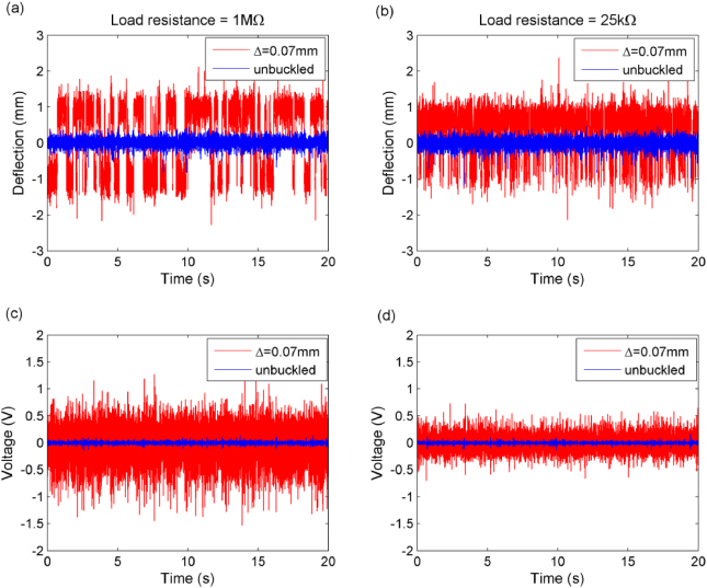
Figure 4. Deflection (above) at the central point and corresponding voltage (below) of the experimental buckled beam against the unbuckled configuration, at 3g of base acceleration, ΔL = 0.07 mm, with load resistance of (a), (c) 1 MΩ and (b), (d) 25 kΩ.
Download figure:
Standard imageIn effect, in figure 4(b), the deflection distribution clearly appears asymmetrical. This is due to the unimorph structure of the experimental laminate, which determines the asymmetry of the potential well. It can be noted that output voltage strongly decreases with decreasing load resistance, while the displacement is only slightly affected. This means that the shunt effect does not affect very much the bistable dynamics of the oscillator.
Figures 5(a) and (b) illustrate the comparison of the rms voltage and the average electrical power respectively versus load variation between linear and nonlinear configurations. In particular, the unbuckled beam is compared to two buckled configurations corresponding to ΔL = 0.05 and 0.07 mm of compression lengths (equivalent to 0.09% and 0.12% of the unbuckled beam length of 55 mm). In this first test, the increasing trends are qualitatively similar for both linear and nonlinear regimes but with a remarkable difference in the amplitude. The maximum rms voltage read from the linear beam is 0.018 V, whereas, it corresponds to 0.095 V and 0.29 V respectively for the first and second buckling cases. In figure 5(b), the average electrical power delivered to the load was calculated by the formula  . What is more important to stress is that the energy harvester in a nonlinear regime is capable of generating one order of magnitude more power than its resonant counterpart, at the same 3g base acceleration. In addition, the optimal load increases from 25 to 150 kΩ in the first buckled example, while for higher compression the power curve keeps increasing for the entire interval. Therefore, the nonlinear nature of buckled systems widens the impedance bandwidth so as to make this configuration more suitable for different operations like battery charging, sensing, radio frequency transmission and sleep mode.

Figure 5. Comparison of (a) rms voltage and (b) power versus load resistance of unbuckled beam with respect to two buckled configurations for ΔL = 0.05 and 0.07 mm.
Download figure:
Standard imageFigures 6(a) and (b) show the standard deviation of the midpoint deflection q(t) = w(L/2,t) over a time interval of ΔT = 20 s versus compression ratio percentage ΔL/L (%). All the experimental quantity are normalized by a constant and expressed in arbitrary units to be comparable with numerical results. Each graph shows three curves relative to different rms noise accelerations, equal to σ = 1–3g. In this test, the standard deviation of the central point deflection is chosen as an indicator to measure the dynamic dispersion around the average equilibrium position in the unbuckled case, which in our case corresponds approximately to zero. In fact, under Gaussian noise this represents a reliable parameter to quantify the strength of the output signal. The same approach has been used for the output voltage in place of the rms not to take into account accidental bias or dc artefacts. As the beam is compressed, the vibration amplitude of the central point increases, achieving a maximum. Close after this critical point, it suddenly falls down to smaller vibration amplitudes which become about half of the unbuckled system. This phenomenon is in good agreement with the bistable dynamics discussed in section 2.2 and previously explained by the authors [17]. Once the barrier height is too high to be climbed within the chosen time interval, the buckled oscillator is confined to vibrate around one of the two minima of the quartic potential well. Therefore, the vibration amplitude is reduced as q ∝ σ/ω± which is due to the stiffening effect, wherein the intrawell resonance  increases. The enhancement of beam deflections with respect to the value at ΔL = 0 mm goes from a factor of 1.5 to 6.7 for the experimental device and from 1.4 to 2.5 for the simulated system. From a qualitative point of view, these ranges can be considered in good agreement. On the other hand, the quantitative mismatch is due to the approximations on the theoretical model which does not fit exactly the real system. Besides, the shaker response was nonlinear at high accelerations.
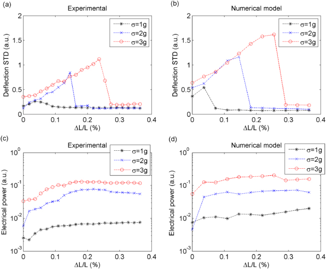
Figure 6. (a), (b) Standard deviation of the beam midpoint deflection q(t) = w(L/2,t) calculated within a time interval of 20 s. (c), (d) Electrical average power versus relative compression ΔL/L (%) for experiment (left column) and numerical simulation (right column).
Download figure:
Standard imageFigures 6(c) and (d) describe the average electrical power versus the compression length ratio respectively for the experimental and numerical models. The average power is calculated here with the formula  , where RL = 1 MΩ is the resistive load and Vstd is the standard deviation of the voltage through it. These results correspond to the aforementioned deflection dynamics. When the beam is compressed the average power increases, with maximum power amplification factors of 2.9, 13.1 and 3.7 at σ = 1 and 3g rms of base acceleration respectively in the experimental case. The numerical model instead gives gain factors of 1.6, 3.9 and 1.9. It is interesting to note that there exists an optimal value of acceleration corresponding to the maximum amplification factor: in this case the intermediate acceleration of 2g. This effect is also predicted by the simulations. Apart from the beam asymmetry, in the first place, the general discrepancies with the theoretical model can be accounted for by the electrode contact leakage of the testing device and, in the second place, to the unknown experimental value of the piezoelectric film elastic stiffness. This parameter was indeed taken equal to 4 × 10¹⁰ Pa by the typical Young's modulus range for thin piezoelectric films [33].
The effective stress–charge piezoelectric coupling was estimated by using the same method of Roundy and Wright [34]. It was found to be equal to ezx =− 0.003 C m−2 which is two orders of magnitude smaller than the theoretical value ezx =− 0.4 C m−2. In addition, the damping ratio was assumed to be constant, whereas in general it depends on the nonlinear tuning force, as also indicated in previous works [35].
Despite discrepancies, the trends are increasing in both cases and they do not exhibit critical breakdown points as in the deflection plots. A possible interpretation of such a phenomenology can be given as follows. Different from piezoelectric coupled equations of previous works [17, 36], the governing equations (17) include the voltage–velocity coupled terms with k1: fifth on the left-hand side of the first equation and first on the right-hand side of the second equation. Being k1/k0 ∼ 104 m−1, the voltage–velocity term that is due to the in-plane piezoelectric force outweighs the piezoelectric coupling term due to the bending. This can be seen in figure 7 where numerical simulations were performed comparing the system response with zero in-plane piezoelectric force (k1 = 0) and with nonzero force (k1 < 0). As this term is proportional to the velocity, when the system passes over the critical bifurcation point, it seem to be responsible for keeping the output voltage high as intrawell vibrations occur at higher frequency. So the absence of a breakdown in the output voltage is qualitatively predicted by the model. Nevertheless, it must be noticed that the power gain results are more important in the experimental data than for simulations.
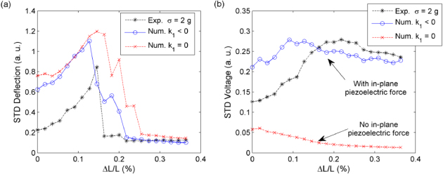
Figure 7. Comparison of numerical model response against experimental data, at 2g rms acceleration base, with (k1 < 0) and without (k1 = 0) the axial in-plane piezoelectric force term for (a) deflection and (b) voltage, respectively.
Download figure:
Standard image4. Conclusions
Theoretical analysis and experimental investigations on a piezoelectric buckled beam used as a vibration energy harvester have been successfully carried out along with numerical simulations. The governing equations of the system have been determined and discussed. A piezoelectric prototype has been realized by screen-printing low-curing-temperature PZT films on a steel beam support. The energy harvesting performances have been studied when compressing the clamped–clamped piezoelectric beam in order to compare the behaviour of a nonlinear bistable against linear unbuckled dynamical regime. According to previous works, when excited by a wide bandwidth Gaussian noise, the system prototype exhibits an enhancement both in oscillation amplitude and in the output power delivered to a resistive load. Such a behaviour is also qualitatively confirmed by the numerical model.
Moreover, the piezoelectric beam produces up to an order of magnitude more electric power when it is compressed than in the unbuckled case. In particular, a gain of 13.1 times was found for an intermediate base acceleration level, which in our case is 2g. It means that there exist no direct proportionality between gain and acceleration. Contrary to intuitive expectations, like in previous magneto-elastic bistable systems [17, 31], the system reveals that, after the bifurcation point, the breakdown in the rms voltage does not occur. This could be interpreted as due to the dependence of electromechanical coupling on the oscillation frequency combined with the high-pass filtering effect. The experimental system has also been studied when varying the resistive load confirming the improvement of electrical performance compared to a linear resonant system. Investigations of such a buckling method to electromagnetic and capacitive conversion methods are indeed envisaged. Micro-scale piezoelectric generators based on the buckling approach can also be considered with the same theoretical approach developed here.
Acknowledgments
This work was carried out under the European FP7 NanoPower project. Useful discussions with Professors P Basset and M Amri of ESYCOM Lab at ESIEE, Université Paris-Est, are gratefully acknowledged.