
Abstract
The design of vibration energy harvesters (VEHs) is highly dependent upon the characteristics of the environmental vibrations present in the intended application. VEHs can be linear resonant systems tuned to particular frequencies or nonlinear systems with either bistable operation or a Duffing-type response. This paper provides detailed vibration data from a range of applications, which has been made freely available for download through the Energy Harvesting Network's online data repository. In particular, this research shows that simulation is essential in designing and selecting the most suitable vibration energy harvester for particular applications. This is illustrated through C-based simulations of different types of VEHs, using real vibration data from a diesel ferry engine, a combined heat and power pump, a petrol car engine and a helicopter. The analysis shows that a bistable energy harvester only has a higher output power than a linear or Duffing-type nonlinear energy harvester with the same Q-factor when it is subjected to white noise vibration. The analysis also indicates that piezoelectric transduction mechanisms are more suitable for bistable energy harvesters than electromagnetic transduction. Furthermore, the linear energy harvester has a higher output power compared to the Duffing-type nonlinear energy harvester with the same Q factor in most cases. The Duffing-type nonlinear energy harvester can generate more power than the linear energy harvester only when it is excited at vibrations with multiple peaks and the frequencies of these peaks are within its bandwidth. Through these new observations, this paper illustrates the importance of simulation in the design of energy harvesting systems, with particular emphasis on the need to incorporate real vibration data.
Export citation and abstract BibTeX RIS
1. Introduction
Energy harvesting (also known as energy scavenging) is the conversion of ambient energy present in the environment into electrical energy for the purpose of powering autonomous wireless electronics systems [1]. Kinetic energy harvesting involves the conversion of environmental vibrations and movements into electrical energy [2]. A kinetic energy harvester typically consists of a mechanical structure that couples the environmental kinetic energy to an electro-mechanical transducer that produces the electrical energy. Power conditioning electronics and some form of energy storage (e.g. battery or supercapacitor) are also normally required. In order to effectively couple the environmental kinetic energy to the transducer, the mechanical structure within the harvester must be carefully designed to match the characteristics of the environmental kinetic energy. A common approach is to match the resonant frequency of the harvester to a characteristic frequency present in the environmental vibrations. This means the optimum solution for harvesting vibration energy from an industrial machine will be different from a harvester designed to capture energy from human motion. Whilst there is considerable worldwide research effort in this topic, much of this work was carried out without considering the characteristics of the kinetic energy found in practical applications. As a result, many publications present novel innovations, but the harvesters themselves have little practical application [3–5].
Previous papers have provided general information regarding vibration levels in certain scenarios. Roundy et al [6] provided a table of acceleration magnitude and frequency of the fundamental vibration mode in a number of applications ranging from cars to buildings. A survey by Miller et al [7] provides the three frequency peaks with the highest acceleration for HVAC and water systems. Vibration data in traffic tunnels has also been presented by Wischke et al [8] and helicopter vibrations by Zhu et al [9]. Since real vibrations typically contain multiple peaks at different frequencies that can be time varying, stochastic or a combination of these, such general headline vibration information omits vital characteristics of the application vibrations.
This paper presents a detailed review of real vibration data from a variety of potential applications. Variations in acceleration, in both time and frequency domains, characterize a given environment and are quantified using data collected over periods of up to 24 h. Such characterizations are key practical considerations that have a significant impact on the design and type of harvester used in a particular application. To demonstrate this, the vibration data has been used to analyse the power output that could be obtained from linear and nonlinear vibration energy harvester systems. For example, a linear resonant harvester with a fixed characteristic frequency can be used in an application where the characteristic ambient frequency remains constant. In such a case, a high-Q, narrow bandwidth, linear harvester producing a high peak power would be most suitable. However, should the ambient frequency change, the output power could reduce dramatically depending upon the Q-factor of the harvester. Small changes in ambient frequency may be accommodated by a wider bandwidth low Q-factor harvester. More significant changes in ambient frequency could require a tunable solution that can track the ambient frequency [10]. Alternatively, in some applications a harvester that exhibits nonlinear behaviour (e.g. bistability [11]) may deliver the most energy.
In order to identify the most suitable type of harvester for a particular application, this paper presents an analysis for different energy harvesters (high-Q linear, low-Q linear, bistable and Duffing-type oscillator) when used in the application scenarios where the vibration data was captured. This analysis is done using C-based simulations that provide a prediction of the total energy harvested over a given time period by each of the different energy harvester types. Both electromagnetic and piezoelectric energy transduction mechanisms have been simulated in this way. The results provide a comparison between the types of energy harvester but it is important to note for reasons discussed in section 5 the objective is not to compare the different transducers. The validity of the simulation results have been indicated through the close correlation between simulation and experimental results of a piezoelectric harvester excited by vibrations from a helicopter.
In conjunction with the summary presented here, a database of raw vibration data in the time domain and analysis in the frequency domain has also been made openly available for the research community via the Energy Harvesting Network's online data repository [12].
2. Models of different types of energy harvesters
This section presents the models of linear bistable and Duffing-type nonlinear configurations for two types of transducer: electromagnetic and piezoelectric. A simulation tool programmed using C language has been used to describe the energy harvester and its electrical load (a resistor in this case) as an integrated model, enabling close mechanical–electrical interaction to be accurately simulated. The simulation approach used in this paper is the same as previously demonstrated in [13] for simulating an entire vibration energy harvester (VEH) system. The only difference is that the tool used in this paper was programmed in C rather than VHDL-AMS as in [13] to reduce the simulation time. The approach has been validated by experimentation and this is presented in section 2.1.5.
2.1. Model descriptions
2.1.1. Linear electromagnetic energy harvester.
The electromagnetic energy harvester design considered is based on a cantilever structure developed by Beeby et al [14]. The coil is fixed to the base, and four magnets located on both sides of the coil form the proof mass (figure 1).
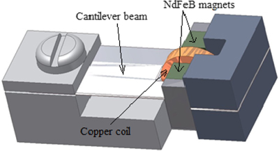
Figure 1. Electromagnetic energy harvester [14].
Download figure:
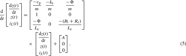
Standard image High-resolution imageThe dynamic model of the energy harvester is given by:

where m is the proof mass, z(t) is the relative displacement between the mass and the base, cp is the parasitic damping factor, ks is the effective spring stiffness, Fem is the electromagnetic force and A is base acceleration. The electromagnetic voltage generated in the coil is given by:

where Φ = NBl is the magnetic flux through the coil and N is the number of coil turns, B is the magnetic field and l is the effective length. The output voltage is defined by:

where Rl is load resistance, Rc and Lc are the resistance and inductance of the coil respectively and iL(t) is the current through the coil. The electromagnetic force is calculated as:

The above equations can be rearranged and written in state-space form (5) to accelerate the simulation speed by using the explicit integration methods described in [15].
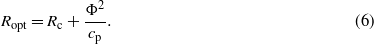
The optimal load resistance is given by [2]:
The parameter values of the electromagnetic energy harvester used in the simulations presented in this paper are listed in table 1.
Table 1. Numerical parameters used in electromagnetic model.
| Symbol | Value | Unit |
|---|---|---|
| m | 2.0 × 10⁻³ | kg |
| N | 6000 | |
| B | 0.45 | T |
| cp (high Q) | 1.3 × 10⁻³ | N m−1 s−1 |
| l | 1.3 × 10⁻³ | m |
| Rc | 4500 | Ω |
| Lc | 0.58 | H |
| cp (low Q) | 3.9 × 10⁻³ | N m−1 s−1 |
The spring stiffness, ks, was chosen according to the measured vibration frequency in each application so that the cantilever's resonant frequency always matches the input centre frequency. The parasitic damping cp determines the Q factor of an energy harvester. In the following simulations, the optimal load condition is always met. This is achieved by calculating cp from the following equation (9). The Q factor of a energy harvester is Q = 1/2ξ, where ξ is the total damping ratio i.e. the sum of electrical damping ratio ξe and parasitic damping ratio ξp:

where  is the resonance frequency. Substituting equation (6) into (7) yields:

where X = 2mωnξ. The positive root of equation (8) is:

Equation (9) is used to control the Q factor in the following simulations of electromagnetic energy harvesters.
2.1.2. Linear piezoelectric energy harvester.
Roundy et al [16] reported a piezoelectric energy harvester based on a two-layer bender (figure 2).
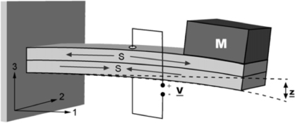
Figure 2. Piezoelectric energy harvester [16].
Download figure:
Standard image High-resolution imageThe detailed design description and deduction of model equations are omitted here due to space limitations; however, the resulting system equations in state-space form are:
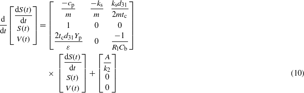
where S(t) is the strain, V(t) is output voltage, d31 is piezoelectric coefficient, tc is the thickness of the piezoelectric layer, Yp is the Young's modulus of the piezoelectric material, ε is the dielectric constant, Cb is the capacitance of the bender and k2 is the strain to displacement ratio (z(t) = k2S(t)).
The electrical damping coefficient is given by [16]:
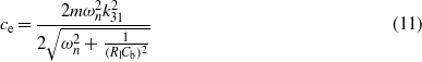
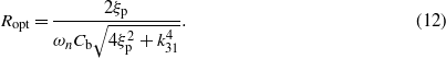
where  is the piezoelectric coupling coefficient. The optimal load resistance is [16]:
The parameter values of the piezoelectric energy harvester used in the simulations presented in this paper are listed in table 2.
Table 2. Numerical parameters used in piezoelectric model.
| Symbol | Value | Unit |
|---|---|---|
| m | 2.0 × 10⁻³ | kg |
| tc | 0.09 × 10⁻³ | m |
| d31 | −100 × 10−12 | m V−1 |
| Yp | 60 × 109 | N m−2 |
| ε | 3 × 10⁻⁸ | F m−1 |
| k31 | 0.14 |
Similarly, ks is chosen according to the measured vibration frequency so that the cantilever's resonant frequency always matches the input centre frequency. The optimal load resistance does not lead to ce = cp. Substituting equation (12) into (11) and substituting the resulting equation into (7) yields:

Equation (13) can be solved numerically for ξp and is used to control the Q factor in the following simulations of piezoelectric energy harvesters. It is observed that ξp = ξ/2 is not a root of equation (13).
2.1.3. Bistable configuration.
Ferrari et al [11] have developed a bistable configuration of the cantilever-based design shown in figure 1. The energy harvester was reported to have a wider bandwidth than the linear configuration, and is therefore an attractive solution for practical energy harvesting applications. Bistability is achieved by attaching one permanent magnet to the tip of the cantilever and one permanent magnet to a fixed end along the beam axis. The two magnets are of opposing polarity, as shown in figure 3.

Figure 3. Bistable cantilever configuration.
Download figure:
Standard image High-resolution imageThe overall nonlinear spring stiffness, kNL, is given by:

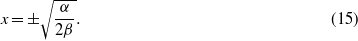
where α and β are constants depending on the distance between the two magnets. For the system to show bistability, α and β need to be chosen as α > ks and β > 0. The stable fixed points created by the magnetic potential wells are at [17]:
The barrier of potential (the level of input vibration above which the proof mass starts to flip between the two potential wells) is given by [17]:
2.1.4. Duffing-type nonlinear configuration.
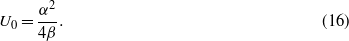
In the above nonlinear spring stiffness equation, if α = 0 and β < 0, the resulting system will behave nonlinearly and also have a wider bandwidth [11]. This is a Duffing-type nonlinear configuration. Figure 4 shows the simulated output power from a nonlinear piezoelectric energy harvester. The linear spring constant is 505.3 which leads to the linear resonant frequency of 80 Hz. The nonlinear spring factor β =− 106, − 5 × 10⁶ and −107 N m−3. It is found that the bandwidth of the nonlinear generator increases with the decreasing β (increasing nonlinearity) although the peak output power is reduced.
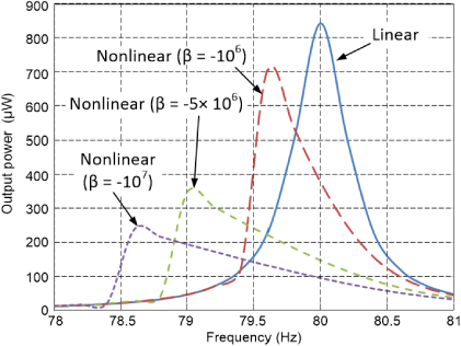
Figure 4. Simulated output power from a nonlinear energy harvester.
Download figure:
Standard image High-resolution image2.1.5. Validation of simulations.
To illustrate the validity of the models, the simulation output was compared with experimental results of a practical energy harvester. A piezoelectric energy harvester was excited using data collected from real helicopter vibrations, and connected through a diode bridge to charge a supercapacitor of 90 mF. The device was a conventional linear harvester and a detailed description and experimental measurements can be found in [9]. The experiments compared the charge rate of the supercapacitor when the harvester was driven by helicopter vibrations replicated on a shaker, and a pure sine wave. The experimental results have been compared to the results from the C-based simulations using the same input excitations.
The pure sine wave vibrations have an amplitude of 0.4 g (1 g = 9.81 m s−2) and frequency of 67.5 Hz, which matches a resonant peak in the helicopter vibration spectrum (to be shown later in figure 12). The simulation and experimental results of charging curves are shown in figure 5.

Figure 5. Simulation and experimental results of charging a 90 mF capacitor.
Download figure:
Standard image High-resolution imageBoth the experimental and simulation results show that the pure sine wave charges the supercapacitors faster than real vibration data. The final supercapacitor voltage for the pure sine wave is also greater than that obtained with the helicopter vibrations. This is because vibration peaks at frequencies other than the resonant frequency can reduce output power of a linear energy harvester [18]. In all cases, the supercapacitor appears to be charged faster in simulation than in practice. This is because the simulation does not consider practical effects such as capacitor leakage and other parasitic losses. Furthermore, in the case of the helicopter vibration the practical experiment does not precisely replicate these vibrations and therefore the excitation achieved in practice is different to that simulated. Hence the charging rate is slower.
In addition, the simulation assumes that the energy harvester has a fixed resonant frequency that always matches the frequency of vibration. However, in the experimental case, the electrical damping of the energy harvester is affected by the voltage on the supercapacitor. As a result, the resonant frequency of the energy harvester shifts from its original resonant frequency and no longer precisely matches the vibration frequency. Therefore the experimental final voltage is lower than simulation results.
3. Case studies
In this section, the energy that can be harvested from the different types of energy harvesters (linear, bistable and Duffing-type nonlinear) under various real vibrations is estimated using the models described in section 2. Two types of transduction mechanism are investigated: electromagnetic and piezoelectric. To be more specific, eight different types of energy harvesters were considered in the simulation. They are linear electromagnetic with high Q, linear electromagnetic with low Q, electromagnetic bistable, electromagnetic Duffing nonlinear as well as linear piezoelectric with high Q, linear piezoelectric with low Q, piezoelectric bistable, piezoelectric Duffing nonlinear.
Two data collection tools were used to sample vibration data at 2048 Hz, a calibrated PCB Piezotronics 354C03 triaxial accelerometer (referred to as 'Tool A'), and an ADXL325 accelerometer (referred to as 'Tool B'). Acceleration data were concurrently collected from the same application using both tools, and found to be comparable. Vibration/movement data were collected from a wide variety of environments and applications, as summarized in table 3. Data was taken from the axis with the highest average acceleration level that would give the maximum output power from a harvester. Raw or processed data from the environments shown in table 3 as well as the measurement setup can be downloaded and found from the Energy Harvesting Network's data repository [12].
Table 3. Overview of vibration data by application.
| Application | Measurement locations | Duration of data | Peak acc. freq. range (Hz) | Acc. range (mg) | Av acc. (mg) | Optimum axis | Tool |
|---|---|---|---|---|---|---|---|
| Car (Ford Focus 1.6 l petrol) | Top of engine | 45 min | 20–190 | 100–1300 | 538 | Normal to road | A |
| Shock absorber mount | 45 min | 10–30 | 5–50 | 18.4 | Normal to road | ||
| Van (VW Transporter, 2.4 l diesel) | Top of engine | 10 min | 30–200 | 370–4190 | 1243 | Front to back | B |
| Dashboard | 7.2 min | 23–85 | 30–300 | 69 | Normal to dash | ||
| Wheel hub | 5 min | 25–325 | 1–1000 | 111 | Tangential to wheel | ||
| Vehicle ferry | Engine | 24 h | 48–50 | 100–1050 | 566 | Perpendicular to drive shaft | A |
| Helicopter | Vertical stabilizer | 20 s | 15–100 | 200–2000 | 257 | Perpendicular to stabilizer | Other |
| CHP plant hot water pump | Pump mounting flange | 24 h | 210–219 | 200–700 | 300 | Parallel to pump shaft | A |
| Clifton suspension bridge | Vertical support from chain to rail | 4 min | 22–46 | 4–40 | 13.6 | Along the length of the bridge | B |
| Ward-Leonard induction motor | Top of motor | 4 min | 50 | 370–399 | 294 | Y axis | A |
| Microwave | Microwave side | 5.4 min | 200 | 280–325 | 287 | Y axis (front to back) | A |
| Washing machine | Front of machine | 1.33 h | 25–192 | 5–230 | 12 | Z axis (normal to machine front) | A |
To illustrate the value of using real vibration data when designing, selecting and simulating energy harvesting system, this section considers five different case studies—four or which use real vibration data (a ferry engine, a combined heat and power (CHP) plant pump, a car engine, and a helicopter), and one considering white noise vibration. The remainder of this section presents and analyses the data obtained from these case studies.
3.1. Vehicle ferry engine
Vibration data was collected from a 4 stroke 8 cylinder diesel engine on Red Funnel's 'Red Osprey' vehicle ferry, which operates between Southampton to the Isle of Wight. The ferry is 93 m long and can carry 220 cars [19]. The Stork-Wärtsilä diesel engine, produced in 1994, can deliver 1207 kW power, a maximum speed of 779 rpm and has had approximately 16 500 h use. The engine is connected to a Voith-Schneider propulsion system which provides both propulsion and steering control. The engine is operated at a small number of different constant speeds which can be selected from the bridge. The ferry runs continually apart from a 2 h period between the last trip of the day and the first trip of the next day. The ferry spends 30–35 min loading and unloading in each port and takes approximately 55 min to make a single crossing.
To collect acceleration data, the accelerometer was mounted on the side of the engine with the x and y axes perpendicular and parallel to the drive shaft respectively and the z axis normal to the deck. A plot of mean acceleration versus frequency is given in figure 6, showing a clear peak at 48 Hz for both the x and z axes. This is a snapshot of a 1s FFT and was taken when the peak vibration amplitude was at the maximum point measured over the complete test. The complete data information can be found in [12]. The times when the ferry was making the crossing can clearly be seen through inspection of the data shown in figure 7, when the magnitude of the acceleration reaches around 1 g with a clear characteristic frequency at 48 Hz. On one occasion (the final trip of the day) the engine speed was at a higher setting providing a dominant vibration at 50 Hz and with a lower magnitude. When the ferry was in port and the engine was idling, the acceleration levels fell to approximately 150 mg with no dominant frequency.
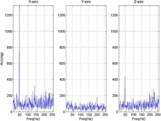
Figure 6. Acceleration levels in the frequency domain for the car ferry.
Download figure:
Standard image High-resolution image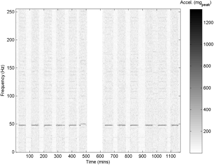
Figure 7. Plot of peak acceleration frequencies along x axes over a long term period on the car ferry.
Download figure:
Standard image High-resolution image3.2. CHP pump
CHP systems cogenerate electrical power and heat locally for particular buildings. The data presented here was collected from the district hot water circulation pump located at the University of Southampton's Highfield Campus. The pump speed is controlled in order to maintain a constant pressure in the system, and the controller was operating a higher loading in the winter. The accelerometer was mounted on the coupling flange of the pump with the z axis parallel to the pump shaft. The vibrations were monitored for a period of 24 h and the plot of average acceleration levels versus frequency for the 3 axes is given in figure 8. The FFT was calculated using 1 s of data for the 24 h period of the test. Figure 8 shows clear resonances at 18 and 211 Hz in all three axes. However, a plot of the discrete FFT results versus time for the z axis, as shown in figure 9, highlights some important practical information. The characteristic frequency with the highest acceleration (the darkest trace in figure 9) is unstable and varies between 209 and 219 Hz over the 24 h period, with a variation of 5%.

Figure 8. Acceleration levels in the frequency domain for the CHP pump.
Download figure:
Standard image High-resolution image
Figure 9. Plot of peak acceleration frequencies along z axes over the 24 h period on a CHP.
Download figure:
Standard image High-resolution imageThis rate of change is typically gradual with a reduction of 9 Hz, for example, taking place over 7.5 h. The fastest change in frequency occurs after 16.6 h when the frequency increases from 210 to 219 Hz in 14 min. These values correspond to the pump speed varying due to changes in pressure as valves open and close in the heating system. In winter the pump is running at around 80–85% of the full speed, whilst in summer this value reduces to around 60% with much smaller changes in the peak characteristic frequency of around 3 Hz or 1.5%. The acceleration level varies substantially over the 24 h from 200 to 700 mg with an average value of 300 mg.
3.3. Ford Focus 1.6 l petrol engine
The vibrations produced by a car engine vary depending upon the engine revolutions and load. These are dependent upon the vehicle's speed, gear and factors such as inclines and acceleration. Measurements were obtained on a 1.6 l Ford Focus petrol engine mounted transversely in a front wheel drive car. The accelerometer was attached to a custom bracket mounted on top of the engine block. The bracket and accelerometer were modelled using finite element analysis to ensure its resonant frequencies were different from the frequency range of interest. The x axis was aligned along the length of the car (front to back), the y axis was aligned parallel to the drive shafts and the z axis was normal to the surface of the road. Vibrations were monitored for the duration of a 28 mile commute beginning at 8:45 am in typical traffic conditions. The journey combined rural country roads, motorway and city driving. Engine parameters such as load and rpm were continually logged and car location and speed tracked using GPS for the entire journey. This enables particular vibration levels to be precisely attributed to particular driving conditions.
A plot of average acceleration versus frequency is given in figure 10, showing that for all 3 axes there is a peak frequency at 80 Hz. However, when plotting the acceleration amplitude and peak frequency in the time domain for the 3 axes (figure 11), there is clearly a considerable variation in the peak acceleration frequency. In the x axis the peak acceleration frequency varies from around 20 up to 190 Hz with occasional peaks around 245 Hz. There is no clear correlation between the x axis vibrations and the driving conditions. There is much less variation in the y and z axes and a clear correlation between the driving conditions and the vibrations. In the y and z axes the peak acceleration frequency varies from around 20 to 120 Hz. This reduced range is explained by the transverse engine configuration with the engine being less rigidly mounted in the x direction. The z axis measurements show a clear correlation between, for example, road speed and acceleration level. From 30 to 39 min into the journey the vehicle is travelling on the motorway at between 63 and 68 mph and the acceleration level is consistently higher for this part of the journey. Periods of town driving are also clearly distinguishable, for example during the first five minutes, from 19 to 24 min and for the final 6 min of the journey after leaving the motorway. As expected, the peak acceleration frequency during these parts of the journey is much more varied and the acceleration levels reduce in comparison with the x axis.
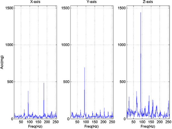
Figure 10. Acceleration levels in the frequency domain for the 1.6 l petrol engine.
Download figure:
Standard image High-resolution image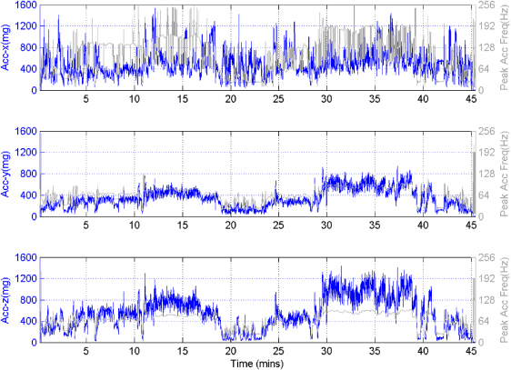
Figure 11. Acceleration level and peak acceleration frequency in the time domain for x,y and z axes on the 1.6 l petrol engine.
Download figure:
Standard image High-resolution image3.4. PZL-SW4 helicopter
Figures 12 and 13 show vibration data obtained from the vertical stabilizer on a PZL SW-4 helicopter, in both the frequency and time domains respectively. The helicopter was flying horizontally at 200 km h−1 and at an altitude of 1000 m with an outside air temperature of 10.5 ° C. The main rotor was rotating at 7.51 Hz. The data was acquired and provided by PZL and has been collected over a shorter period of time (20 s). The vibration spectrum clearly shows multiple peaks at different frequencies and these are stable with time because the rotor speed is constant. These vibration frequencies are replicated over the airframe and, together with the vibration amplitudes, this presents a good energy source for vibration energy harvesting.

Figure 12. Acceleration levels in the frequency domain for the SW-4 helicopter.
Download figure:
Standard image High-resolution image
Figure 13. Acceleration level in the time domain for the SW-4 helicopter.
Download figure:
Standard image High-resolution image3.5. White noise vibration
Figures 14 and 15 show the spectrum and time signal of white noise acceleration, respectively. The time-domain signal was generated in Matlab and, as expected, its spectrum shows no obvious dominant components. The vibration acceleration was set to the level that allowed the bistable structure to always operate in bistable operation.
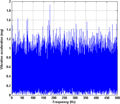
Figure 14. Spectrum of white noise vibration.
Download figure:
Standard image High-resolution image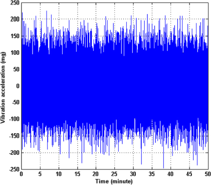
Figure 15. Time signal of a white noise vibration.
Download figure:
Standard image High-resolution image4. Simulation results
In this section, simulation results are presented for the average output power of a linear energy harvester with a high Q, a linear energy harvester with a low Q, a bistable energy harvester and a Duffing-type nonlinear energy harvester, when excited by the vibration sources presented in section 3.5
In order to provide a fair comparison, assumptions are made for all simulations. Each energy harvester has a proof mass of 2 g. For the linear energy harvester, its resonant frequency always matches the peak frequency or one of the peak frequencies of the input vibration. For the white noise input, the resonant frequency of the linear energy harvester was chosen arbitrarily to be 200 Hz. This is because white noise has a flat power spectral density and the simulation result is independent from the selection of the resonant frequency. For the bistable energy harvesters, the stable fixed points are set to be around ±2 mm. Using equations (15) and (16), values of α and β were chosen to satisfy α > ks and β > 0 while maintaining the lowest level of potential barrier. For the Duffing-type nonlinear energy harvesters, β has been chosen as −1 × 10⁷, i.e. only soft nonlinearity is considered in this simulation. The frequency at which the peak power is achieved is set to match the resonant frequency of the linear energy harvester. The load resistance is always optimal, i.e. the power delivered to electrical load is maximized.
Table 4 lists the simulation results for electromagnetic energy harvesters. The load resistance, electrical and total damping ratio, α and β values of the bistable and nonlinear energy harvesters are also listed in the tables. Please note that the parasitic damping ratio, ξp, is a function of the resonant frequency for electromagnetic energy harvesters according to equation (9). As the resonant frequency is different in each case, ξp is different and therefore the electrical damping ratio, ξe, also varies in different cases.
Table 4. Simulation results of different types of electromagnetic energy harvesters.
| Vibration data (duration/centre freq.) | Linear high Q (Q = 300,ξ = 0.0017) | Linear low Q (Q = 100,ξ = 0.005) | Bistable (Q = 100,ξ = 0.005) | Duffing-type nonlinear (Q = 100,ξ = 0.005) | |||||||||||
|---|---|---|---|---|---|---|---|---|---|---|---|---|---|---|---|
| Rl (kΩ) | ξe | E (mJ) | Rl (kΩ) | ξe | E (mJ) | Rl (kΩ) | ξe | α | β | E (mJ) | Rl (kΩ) | ξe | β | E (mJ) | |
| White noise (50 min/200 Hz) | 6.2 | 0.0007 | 672 | 2.8 | 0.0012 | 329 | 2.8 | 0.0012 | 5750 | 7.19 × 10⁸ | 349 | 2.8 | 0.0012 | −1.0 × 10⁷ | 329 |
| Car engine z-axis (45 min/96.3 Hz) | 8.4 | 0.0004 | 423 | 5.6 | 0.0005 | 130 | 5.6 | 0.0005 | 1000 | 1.25 × 10⁸ | 34 | 5.6 | 0.0005 | −1.0 × 10⁷ | 137 |
| Car engine x-axis (45 min/79 Hz) | 9.4 | 0.0005 | 125 | 5.9 | 0.0006 | 40 | 5.9 | 0.0006 | 575 | 7.19 × 10⁷ | 25 | 5.9 | 0.0006 | −1.0 × 10⁷ | 37 |
| Ferry engine x-axis (100–200 min/48 Hz) | 13.5 | 0.0006 | 31 455 | 7.0 | 0.0009 | 7127 | 7.0 | 0.0009 | 375 | 4.69 × 10⁷ | 179 | 6.8 | 0.0009 | −1.0 × 10⁷ | 737 |
| CHP z-axis (950–1050 min/211 Hz) | 6.1 | 0.0002 | 431 | 5.0 | 0.0003 | 93 | 5.0 | 0.0003 | 3500 | 4.38 × 10⁸ | 3 | 5.0 | 0.0003 | −1.0 × 10⁷ | 93 |
| Helicopter vibration (50 min/67.5 Hz) | 10.4 | 0.0005 | 3 243 | 6.2 | 0.0007 | 817 | 6.2 | 0.0007 | 500 | 6.25 × 10⁷ | 318 | 6.2 | 0.0007 | −1.0 × 10⁷ | 403 |
Table 5 lists the simulation results for piezoelectric energy harvesters. In this case, ξp was calculated using equation (13) and is only a function of total damping ratio, ξ. It was assumed that the total damping is the same in all cases and therefore, ξp and ξe are the same in all cases.
Table 5. Simulation results of different types of piezoelectric energy harvesters.
| Vibration data (duration/centre freq.) | Linear high Q (Q = 300,ξ = 0.0017) | Linear low Q (Q = 100,ξ = 0.005) | Bistable (Q = 100,ξ = 0.005) | Duffing-type nonlinear (Q = 100,ξ = 0.005) | |||||||||||
|---|---|---|---|---|---|---|---|---|---|---|---|---|---|---|---|
| Rl (kΩ) | ξe | E (mJ) | Rl (kΩ) | ξe | E (mJ) | Rl (kΩ) | ξe | α | β | E (mJ) | Rl (kΩ) | ξe | β | E (mJ) | |
| White noise (50 min/200 Hz) | 4.6 | 0.0008 | 1 107 | 13.0 | 0.0024 | 1 070 | 13.0 | 0.0024 | 5750 | 7.19 × 10⁸ | 2549 | 13.0 | 0.0024 | −1.0 × 10⁷ | 1070 |
| Car engine z-axis (45 min/96.3 Hz) | 5.4 | 0.0008 | 856 | 15.2 | 0.0024 | 683 | 15.2 | 0.0024 | 1000 | 1.25 × 10⁸ | 354 | 15.2 | 0.0024 | −1.0 × 10⁷ | 748 |
| Car engine x-axis (45 min/79 Hz) | 5.6 | 0.0008 | 197 | 15.8 | 0.0024 | 158 | 15.8 | 0.0024 | 575 | 7.19 × 10⁷ | 144 | 15.8 | 0.0024 | −1.0 × 10⁷ | 146 |
| Ferry engine x-axis (100–200 min/48 Hz) | 6.3 | 0.0008 | 27 432 | 17.8 | 0.0024 | 13 975 | 17.8 | 0.0024 | 375 | 4.69 × 10⁷ | 908 | 17.6 | 0.0024 | −1.0 × 10⁷ | 1565 |
| CHP z-axis (950–1050 min/211 Hz) | 4.7 | 0.0008 | 2 808 | 13.3 | 0.0024 | 1 645 | 13.3 | 0.0024 | 3500 | 4.38 × 10⁸ | 66 | 13.3 | 0.0024 | −1.0 × 10⁷ | 1646 |
| Helicopter vibration (50 min/67.5 Hz) | 5.8 | 0.0008 | 3 837 | 16.4 | 0.0024 | 2 375 | 16.4 | 0.0024 | 500 | 6.25 × 10⁷ | 1258 | 16.4 | 0.0024 | −1.0 × 10⁷ | 1336 |
5. Discussions
The purpose of this comparison is to compare linear, bistable and Duffing's nonlinear structure for each particular transducer. It is not the intention to compare the electromagnetic and piezoelectric transducers. Therefore, electromagnetic and piezoelectric energy harvesters are discussed separately. This is because the output power of both electromagnetic and piezoelectric energy harvesters depends on many variables such as magnetic field strength and coil dimensions for electromagnetic energy harvesters and d31 and k31 coefficients for piezoelectric energy harvesters. The values of these variables used in the simulation were based on previous designs and typical values. For these values, under the optimal load conditions, the energy coupled to the electrical load for electromagnetic energy harvesters is lower than the piezoelectric case for the same Q factor. This is because the coil in the electromagnetic energy harvester modelled here has a relatively high resistance compared to the optimum load resistance. Therefore, some of the electrical energy converted from the mechanical domain is dissipated in the coil. In this case the piezoelectric energy harvesters can deliver more energy to the load resistance than the electromagnetic energy harvesters. Therefore, since it is not the intention of this study to compare piezoelectric and electromagnetic energy harvesters, conclusions should not be drawn about the relative merits of each approach.
The variables used in the simulation of the bistable and nonlinear generators have been selected to produce a maximum power at the resonant frequency of the linear generator. This enables a straightforward comparison between types of harvester but this approach leaves room for further optimization of variables for particular applications.
Consider the piezoelectric case first. The results show that the linear energy harvester with a high Q has the highest output power and the bistable energy harvester has the lowest output power among the four types of energy harvesters. The exception to this rule is white noise excitation where the bistable approach produces the highest output power. The linear low Q energy harvester and the Duffing-type nonlinear harvester have similar output power levels in all applications. This simulation result is consistent with findings from another research group that show the bistable piezoelectric generator produces more power from white noise excitation [11]. It should be noted that in practice achieving a Q factor of 300 for a piezoelectric harvester is unlikely and the results obtained for the low Q device are more representative of practical implementations. The results do suggest, however, that the Q factor should be maximized and that, for the applications covered here, the reduction in bandwidth is more than offset by the increase in harvester amplitude. This raises the point that another practical limitation of inertial harvesters is the maximum permissible inertial mass displacement which will be limited by the detailed design of the harvester, its material properties and resistance to fatigue. The nature of the input excitation is also a factor and these practical constraints could place a limit on the maximum acceptable Q factor.
However, for electromagnetic transducers, the linear high Q energy harvester produces the highest output power of the four types of energy harvester for all vibration cases. The linear low Q energy harvester and the Duffing-type nonlinear harvester have similar output powers and the bistable type produces the lowest output power in every case apart from the white noise excitation.
Bistable harvesters are better in the white noise case for piezoelectric energy harvester because the electrical energy generated is a function of the stress in the piezoelectric material (i.e. the displacement). At lower frequencies, for a given acceleration level, the vibration amplitude is relatively large. As a result, the proof mass in a bistable structure flips between the two stable positions producing large stresses and high output powers. At higher frequencies, the vibration amplitude for the same acceleration level is lower and the proof mass gets trapped at one potential well. The amplitude of the harvester's vibrations becomes much smaller and the generated power is significantly reduced. This causes the steep drop in its power spectrum as shown in figure 16.
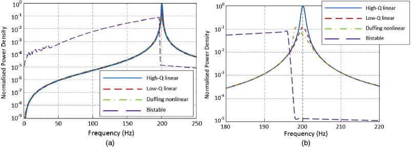
Figure 16. Various piezoelectric energy harvesters' response to white noise. (a) Over a wide frequency range. (b) Near the resonant frequency.
Download figure:
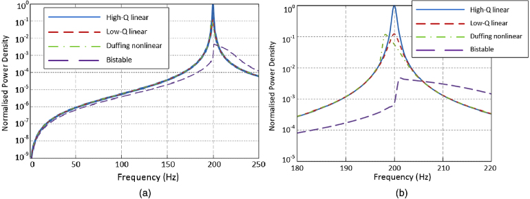
Standard image High-resolution imageIn the case of the electromagnetic energy harvester, the electrical energy generated is mainly a function of the relative velocity of the magnet coil arrangement. For the bistable electromagnetic energy harvester, although the vibration is large enough for the proof mass to travel between the two potential wells at lower frequencies, the output power is low due to the low velocity. Maximum output power from the bistable electromagnetic energy harvester is produced at ∼200 Hz when the velocity the proof mass flips between the two potential wells is maximized. This is the cause of the steep increment in its power spectrum as shown in figure 17. At frequencies beyond this, the bistable harvester becomes chaotic and randomly switches between the two potential wells (rather than at each cycle) with the proof mass becoming increasingly stuck in one potential well as the frequency rises. This is because for a fixed acceleration higher frequencies produce lower amplitudes which are less likely to cause the harvester to switch.
Figure 17. Various electromagnetic energy harvesters' response to white noise. (a) Over a wide frequency range. (b) Near the resonant frequency.
Download figure:
Standard image High-resolution image
When comparing bistable piezoelectric and electromagnetic energy harvesters, another factor to be considered is the level of parasitic damping. Higher parasitic damping (such as in the electromagnetic case compared to a piezoelectric harvester) means more energy is required to trigger the bistable oscillation. Therefore, less output power can be produced by the bistable electromagnetic energy harvester.
Furthermore, it is also found that the low-Q linear energy harvester has higher or similar output power compared to the Duffing-type nonlinear energy harvester with the same Q factor in most of the cases, regardless of the transduction mechanism. The only exception is the case of vibrations in z axis of a car engine. The reason is that the vibration spectrum in z-axis of a car engine (as shown in figure 10) contains multiple peaks, each of which covers a relatively large frequency range and has a large acceleration. As the Duffing-type nonlinear energy harvester has larger bandwidth than the linear energy harvester, its total combined output power is higher although its maximum power is lower than that of the linear energy harvester. However, in cases where the target vibration peak is narrowband and no other vibration peaks are covered by the power spectrum of the Duffing-type nonlinear energy harvester, such as ferry engine (x-axis) and helicopter vibrations, its output is significant lower than that of the linear energy harvester. In cases where the target vibration peak is wideband, such as car engine (x-axis) and CHP (z-axis) vibrations, the linear energy harvester and the Duffing-type nonlinear energy harvester with the same Q factor have similar amount of output power.
6. Conclusions
This paper presents analytical models of linear, bistable and nonlinear vibration energy harvesters. Two transduction mechanisms were studied, i.e. electromagnetic and piezoelectric. C-based simulations have been performed to the study performance of three types of vibration energy harvesters under practical vibration data taken from a diesel ferry engine, a combined heat and power pump, a petrol car engine and the white noise vibration.
The analysis shows that, regardless of the transduction mechanism, a linear energy harvester with a high Q factor delivers more energy to the optimum load than a linear energy harvester with a low Q factor. A bistable energy harvester has the lowest output power among all energy harvesters in most cases except under white noise vibration. When excited under white noise vibration, a bistable energy harvester has the highest output power compared to the other three types of energy harvesters with the same Q factor. However, it was found that it is better to use piezoelectric transducers rather than electromagnetic transducers in bistable structures under white noise vibrations. The reason is that the output of piezoelectric transducers is a function of stress/displacement of the proof mass. Once the proof mass flips between the two stable positions, large changes in stress, thus high output power, can be achieved. However, the output of electromagnetic transducers is a function of velocity of the proof mass. High velocity cannot always be achieved in a bistable structure especially at lower frequencies. Furthermore, the electromagnetic energy harvesters normally have higher parasitic damping than the piezoelectric energy harvesters, which make bistable transition more difficult to happen.
It is also found that the linear energy harvester has higher output power compared to the Duffing-type nonlinear energy harvester with the same Q factor in cases where the target vibration peak is narrowband and only a single vibration peak is covered by the power spectrum of the Duffing-type nonlinear energy harvester, regardless of the transduction mechanism. In cases where the target vibration peak is wideband, the linear energy harvester and the Duffing-type nonlinear energy harvester with the same Q factor produce a similar amount of output power. Where more than one vibration peak occurs in the range of the Duffing-type nonlinear energy harvester, it produces a higher output power than the linear energy harvester with the same Q factor.
This research has illustrated that design of vibration energy harvesters depends largely on particular applications and this form of simulation is useful for selecting the correct type and transduction mechanism in dedicated applications. Such simulations can also be used to optimize VEH parameters to maximize energy harvested in various applications.
Acknowledgments
This work was supported by EPSRC, UK, grant number EP/G067740/1, 'Next Generation Energy-Harvesting Electronics: Holistic Approach', website: www.holistic.ecs.soton.ac.uk. The authors would also like to thank PZL, Poland (a partner of EU FP7 research project TRIADE, website: http://triade.wscrp.com/) for kindly providing vibration data on a PZL-SW4 helicopter. The authors would like to thank the staff of Red Funnel for allowing access to their ferries for testing.