

Abstract
To explore the flow characteristics of healing agent leaving a vascular network and infusing a damage site within a fibre reinforced polymer composite, a numerical model of healing agent flow from an orifice has been developed using smoothed particle hydrodynamics. As an initial validation the discharge coefficient for low Reynolds number flow from a cylindrical tank is calculated numerically, using two different viscosity formulations, and compared to existing experimental data. Results of this comparison are very favourable; the model is able to reproduce experimental results for the discharge coefficient in the high Reynolds number limit, together with the power-law behaviour for low Reynolds numbers. Results are also presented for a representative delamination geometry showing healing fluid behaviour and fraction filled inside the delamination for a variety of fluid viscosities. This work provides the foundations for the vascular self-healing community in calculating not only the flow rate through the network, but also, by simulating a representative damage site, the final location of the healing fluid within the damage site in order to assess the improvement in local and global mechanical properties and thus healing efficiency.
Export citation and abstract BibTeX RIS
1. Introduction
Fibre reinforced polymer (FRP) composite materials are leading contenders as component materials to improve the efficiency and sustainability of many forms of transport. The arguments for using this material are their superior specific strength and stiffness, as well as a significantly lower density than their metallic counterparts. However, unlike metallic materials, FRPs do not exhibit 'graceful degradation', when subjected to high strain-rate events, but instead dissipate the energy through complex damage mechanisms resulting in significant reductions in mechanical performance and loss of structural integrity.
As a part of ongoing work at Bristol into multi-functional materials, embedded healing capabilities (see figure 1) for autonomous self-healing is under consideration to address the formation of multi-scale damage in advanced fibre reinforced composite materials. The precise healing strategy employed varies with the intended structural application, and the nature and magnitude of the damage. For example, microcapsules [1–3] distributed appropriately may be sufficient to heal initiating defects and arrest slow propagating cracks, while embedded liquid filled hollow glass fibres [4–6] or vascular networks [7–13] are ideal for facilitating the bleeding of healing agent throughout multiple crack planes within large scale damage.

Figure 1. Self-healing approaches.
Download figure:
Standard image High-resolution imageEmbedding a self-healing delivery network, in the form of hollow glass fibres or a vascular network, offers considerable technical and practical challenges since the delivery system may affect the architecture of the laminate and promote the initiation of new damage scenarios. Therefore, in the design concept phase, it is essential to ensure the network placement and delivery potential is optimized, in addition to the optimization of the healing resin to effect repair (i.e. low viscosity, high toughness with a controlled bio-inspired haemostatic reaction, as identified by Trask [15]).
In the situation when the damage size is extensive through the structure (see figure 2(column II), and there is a need to restore full operational capability, a number of key challenges exist to achieve optimized healing efficiency, namely:
- (i)Identification of the key damaged locations and damage connectivity (as potential healing 'highways' to maximize the healing efficiency potential) within the structure/component (see figure 2);
- (ii)identification of the most effective 'healing locations' requiring reattachment and stabilization to maximize load transfer restoration; and,
- (iii)ensuring that sufficient fluid and fluid flow from the delivery network will gain direct access to the damaged region before polymerization (thrombosis) of the healing agent has occurred.
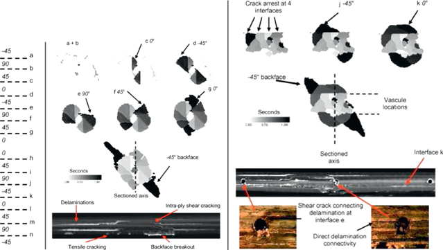
Figure 2. Control 10 J impact damage characterization of baseline and self-healing laminate containing vascules: column I lay-up and interface identification; column II C-scan TOF breakdown (with scale bar for the final image) of baseline specimen; and, column III C-scan TOF breakdown (with scale bar for the final image) and micrographs of damage interaction within a self-healing composite laminate. Adapted from [13].
Download figure:
Standard image High-resolution imageQuantifying the key damaged locations and damage connectivity (point i) has been a key technical driver at Bristol to ensure that the delivery infrastructure (in particular vascular networks) can supply sufficient healing potential to the damage site. This work has been undertaken through linking optical microscopy with ultrasonic c-scanning (for example [6, 13]) and, more recently, micro-x-ray computer tomography μCT [16].
In an effort to address point ii above the reader is directed to our previous work [17], which considered the need for identifying optimum healing locations within the delaminated composite structure to achieve maximum performance restoration; utilising a multi-objective genetic algorithm. The results illustrated the magnitude of attachment (from the top surface to the lower surface) required to ensure effective stabilization of the local crack plane and thus the global damage zone; namely, we reported a fill/attachment ratio of 35% was sufficient to obtain 95% structural efficiency (when the repair of a single delamination loaded in compression was considered) [17]. This result shows the importance of delivering the correct volume of the healing resin to the correct local location within a global damage scenario. Due to the complex damage network observed in fibre reinforced composite (figure 2), it is essential to understand how the liquid flow front permeates through the damage site from a single or multi-point entry strategy.
In the present study, we are assessing the release of the healing fluid from the discreet embedded healing capability (with the aim of addressing point iii above) to ascertain the controlling parameters which determine the rate and extent the healing resin will fully infuse the surrounding damage site. To achieve this objective, a model of the fluid flow leaving the healing reservoir and moving through the damage site is required. Flow of the healing agent into the crack proceeds under the influence of a pressure gradient and/or capillary action. This means these flows involve elaborate geometries, which may even still be in motion, together with free surface behaviour, and potentially also chemical changes in the fluid. Additional complications arise from the need to understand not only a single exit, but potentially a whole network of exit points. Clearly, for the self-healing community there is a great interest in calculating not only the flow rate through the exit, but also the final location of the healing fluid within a crack in order to assess the improvement in mechanical properties.
Although significant progress has been made in the design of self-healing networks, the design and analysis of these systems has proceeded along largely empirical or semi- empirical lines. Experimental data does exist for these low Reynolds number discharge orifices [2, 6], but the benefits of employing numerical modelling would be substantial, potentially delivering not only improved quantitative predictions but also much deeper understanding of the flows in these confined regions, as well as the ability to consider the properties of more complex networks. The flow of self-healing agent exiting a vascule is an example of a free surface flow at a low Reynolds number; at high Reynolds numbers, orifice calculations would give usable results for these problems, but as viscous forces becomes more dominant the behaviour is not as clear. Figure 1(d) shows a PTFE vascule intended to convey healing agent. An important initial question, and one we try to address through the application of smoothed particle hydrodynamics (SPH) (a Lagrangian meshless numerical method for fluid dynamics), concerns determining the link between the local pressure differential across the orifice and the flow rate through it, before the external geometry of the crack is considered.
2. Formulation
SPH was derived independently by Gingold and Monaghan [18] and Lucy [19]. It is often used for fluids due to the simplicity of using meshless methods to model free surface flows which would otherwise require complex techniques such as the volume of fluid (VOF) method [20]. There are a number of reasons to prefer SPH to VOF; the first is simplicity, a basic SPH code can be written with comparative ease and no special techniques are required to track free surfaces. The meshless nature of the method also removes the need to create a mesh which can prove challenging in complex geometries. As the SPH method is Lagrangian it avoids false diffusion errors that can occur in Eulerian methods such as VOF. In addition, VOF requires the solution of a differential equation that describes the evolution of the volume fraction in the mesh volumes which is unnecessary in SPH.
To represent the flow of fluid with a Lagrangian scheme equations (1) and (2) must be solved which requires calculating the derivatives from the primative variables. The most commonly used method for producing SPH formulations of the governing equations views SPH as a method of representing a function by summation over a set of particles. Liu and Liu [21] give details of the mathematics, but the process is to take a function that approximates the Dirac delta function and convolve it with the function to be represented as in equation (3). The angle brackets denote the integral representation


Here  is a function to be represented by integration over a volume Ω,
  is a smoothing function that depends on the difference between the location of interest and the points over which the integral is evaluated.
This integral representation, in equation (3), is then approximated by summation over N nearby particles, shown in equation (4), where each particle is assigned a mass and density such that the volume taken up by the particle can be calculated from these values. This summation is practical because W is usually chosen to be a compact function which is non-zero only for a small fraction of the total domain. The radius over which W is non-zero is known as the support radius and is a function of h, which is a characteristic length of W and is known as the smoothing length. Thus N is the number of particles within the support radius

Derivatives can be approximated in the same way as any other function, and since  is required:

However, as the derivative of f may not be known the following identity can be used to give two terms in the integral, where the term on the left-hand side of equation (6) becomes a surface integral through the gradient theorem, equation (7)

Normally, though not in regions where the support is truncated, the support domain is entirely within the problem domain such that the surface integral is zero and the representation can be expressed entirely in terms of the volume integral. The particle approximation can then be performed as with any other function. The method for deriving the approximation to a vector gradient is very similar.
With this information it possible to construct the governing equations of fluid flow in the SPH formulation as all derivatives can be simply expressed in SPH form

Equation (6) can be used in conjunction with identities to produce expressions for derivatives. An identity using  is given by equation (9), suitable since from equation (1) the variable needed is
  . This has the advantages of being symmetric and consistent with a parallel derivation based on the Lagrangian [22]

Evaluating the derivatives on the right-hand side (using  or
or  ) separately gives the SPH result for
At present the SPH formulation used is:


Equation (11) is the quintic kernel suggested by Wendland [23] and α is a normalization parameter than depends on the dimension the equations are solved in. The normalization is necessary so that the volume integral of the kernel over the support radius is equal to one; this allows the approximation in equation (3). In 2D  while in 3D
  for this kernel. The equation of state, equation (14), is commonly used in SPH remove the need to solve a pressure Poisson equation. An equation of this form was first suggested by Cole [24] for water, Monaghan [25] then suggested setting B such that the speed of sound in the fluid is an order of magnitude greater than the fastest particle. γ is set to 7 following Cole's [24] work. The second term on the right-hand side of equation (12) is a viscosity term, which can be formulated in different ways discussed below. The density of a particle is evolved in time rather than calculated explicitly by summation to remove the problem of the density reducing near free surfaces due to the lower number of near particles [26]. Once the discrete equations have been set up on the particles, Newmark's scheme is used to advance the model in time with iteration applied at each timestep to solve the implicit problem.
2.1. Viscous force formulation
The resins used in the self-healing process often have high viscosity and the length scales in question are low, implying a small Reynolds number. Viscous forces will be significant so an accurate representation of these forces in the SPH model is essential. In this work a viscosity formulation due to Cleary [27] is used. This formulation has two attractive properties. It can allow variable viscosities within a fluid or interactions between fluids of different viscosities, and it was tuned by considering a Couette flow for correlation with experimental data using a tuning parameter. Cleary's formulation is given by equation (15) and the parameter ξ is given by Cleary as equal to 4.963 33
The results obtained using Cleary's viscosity formulation are compared to an alternative formulation suggested by Morris et al [28], given in equation (16). Note that this method does not require a tuned parameter and although similar in appearance, acts in a slightly different direction to the Cleary viscosity term

2.2. Surface tension formulation
There are two main methods for the modelling of surface tension forces within SPH. One method is based upon the work of Brackbill et al [29] where a continuum surface force model (CSF) is used such that the surface forces of surface tension become volume forces, removing the need to accurately track the interface. However, surface curvature must still be calculated. Morris [30] presents the first use of the CSF method applied to SPH and shows a number of methods for calculating the surface tension. While these methods provide good results they rely on a calculation of curvature which can be challenging and typically needs two phases to operate, which is both computationally expensive and contrary to the physics when dealing with fluids in a vacuum.
The second method, used within this work, is formulated as a pair-wise force between particles applied everywhere [31]. The force term is based upon molecular forces; these forces should be repulsive at short ranges, attractive at medium range and decay away to zero for longer ranges. This force term is usually given by equation (17) where the support radius of a particle is equal to  . The coefficient sij sets the strength of the surface tension forces and can vary depending on what phase a fluid particle is interacting with or if it is interacting with a solid boundary. Tartakovsky et al [32] show how this parameter can be related to physical surface tension and contact angle values (see section 4 for the values used in this model)
2.3. Comparison with VOF method
The VOF method is another numerical method often used to model problems with free surfaces. Although no comparison between SPH and the VOF method is performed in this work, a large number of these comparisons have been presented in the literature. Ha et al [33] compare the performance of an SPH code and MAGMAsoft, which uses the VOF method, in predicting the behaviour of a water analogue experiment for gravity die casting. Results are very favourable with both numerical methods predicting the behaviour of the fluid well and SPH better predicting the free surface. The work was later extended to 3D [34], with He et al [35] presenting similar conclusions. Cleary et al [36] build on the work of Ha et al [33] to include heat transfer and solidification effects and again SPH compares favourably to MAGMAsoft using the VOF method. Colagrossi [37] presents a comparison between SPH and a level set method for a number of problems including the deformation of a square patch of fluid under a velocity field, the behaviour of a bubble in a denser fluid and a dam break.
Shao and Lo [38] present a comparison of the results of a dam break test case between experimental data and a number of numerical methods including both SPH and the VOF method. Both methods show good agreement with each other and the experimental results. Further results are reported by Zheng et al [39]. The results of numerical simulations of flow over the blade of a Turgo turbine are presented by Koukouvinis et al [40], showing a comparison between SPH and the VOF method. Good qualitative agreement is seen in the flow fields between the two methods and good quantitative agreement in total torque on each blade.
3. Results
Numerical experiments were conducted to investigate the ability of SPH to simulate fluids of various viscosities being forced from a tube into space through a small nozzle. In the simulation initially there is a cylindrical container with fluid in equilibrium and a piston above it (tank diameter to exit diameter ratio is 6). This replicates a constant driving pressure across the nozzle. Figure 3 shows a 2D version of the configuration of the test and shows how SPH captures the physics of high and low viscosity fluids being forced through the nozzle. Numerical results were matched with experimental results by modifying the viscosity used in the numerical simulations such that the Reynolds number matched experiment.

Figure 3. Fluid exiting 2D tank. Left: low Reynolds number (Re = 3.4), right: high Reynolds number (Re = 5100).
Download figure:
Standard image High-resolution imageTests were conducted without gravity, so a constant force was applied to the piston in order to generate constant driving pressures. An equation of motion was solved to update the position of the piston, with the equation of motion for the piston solved using strong fluid-structure coupling [41], so that a number of fixed point coupling iterations were executed for every timestep until the piston position converged. A Newmark integration scheme was used for both the fluid and piston. The coupling process between the fluid and piston started with an estimate of the fluid solution for timestep  which was then used to supply a force to the piston equation of motion to advance the piston to
  . This new position of the piston was then used to obtain an updated
  fluid state, and the cycle continued until convergence of the
  fluid and piston states.
A range of viscosities were tested in order to explore the relationship between non-dimensional mass flow and the nozzle Reynolds number. For a constant driving pressure the expected physics are seen in the relationship between mass flow rate and dynamic viscosity; for low viscosity the mass flow rate is nearly independent of viscosity as inertial forces dominate, but gradually the viscous forces become more important and a variation of the mass flow rate is clearly seen. In the flow solution a small transient is initially observed but this quickly dies away. The mass flow rate is calculated by taking the gradient of the curve from the time-marching simulation once the initial transient has decayed and the system settled to a steady state.
Figure 4 is the characteristic non-dimensional curve for the geometry. It shows a clear relationship between the discharge coefficient Cdis, (where  v is the mass averaged steady state velocity, and h is the equivalent hydrostatic head) and nozzle Reynolds number. The nozzle reynolds number is defined as
  with D being the nozzle diameter. The limit value of Cdis at high Re is around 0.4, which is somewhat short of the experimental value of 0.62 [42] for a sharp edged orifice owing to ambiguity over the actual orifice width as a result of a coarse particle spacing. Running a high Reynolds number case with a higher particle resolution yields a higher value of 0.6, which is much closer to experimental data. The results obtained with the different viscosity formulations were very similar with no difference in the higher Reynolds number regime as the viscous forces are insignificant, although the Cleary viscosity term gives slightly lower discharge coefficients at lower Reynolds numbers.
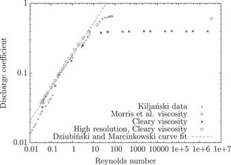
Figure 4. Characteristic curve of discharge behaviour as a function of Re.
Download figure:
Standard image High-resolution imageComparison of these numerical results to experimental data by Kiljański [43], using glycol ( Pa s), glycerin (
 Pa s and
  Pa s) and syrup (
 Pa s), is favourable. Kiljański observed a plateau in Cdis after a Re near to 20, which matches figure 4, and once a higher particle resolution is used the numerical results are a better match to the experimental data at high Reynolds number as discussed above. For low Reynolds number flows (
 ) Kiljański found the experimental regression line
  whereas the low resolution results for this numerical study are fitted by the curve
  demonstrating good performance of the model. The higher resolution results show a higher discharge coefficient for a given Reynolds number than that measured by Kiljański but compare much more favourably to the experimental results of Dziubiński and Marcinkowski [42], who fit the curve
  to their low Reynolds number data, while the high resolution results presented here are fitted by the curve
  Dziubiński and Marcinkowski use water (
 Pa s), glycol (
 Pa s) and starch syrup solutions (
 Pa s–
Pa s– Pa s), (note no attempt is made here to the simulate the non-Newtonian fluids used). The main difference between the results of Kiljański and those of Dziubiński and Marcinkowski seems to be in the calculation of the discharge coefficient. Kiljański used the mean of the head at the beginning and end of discharge while Dziubiński and Marcinkowski used a differential relationship between head and discharge time.
4. Resin filling of crack volume
To explore the ability of the method to predict filling of a crack volume, the geometry shown in figure 5 was modelled in the absence of gravity. This consists of two connected delaminations, of width 30 μm. In order to model the influx of the fluid in to the crack, a reservoir of fluid is positioned at the entry to the crack system, which is driven by a piston moved with a constant force to drive the fluid in to the crack at 1.19 Pa. Since this case involves direct contact between the fluid and cavity walls, it is important to include the influence of surface tension. At these scales it is expected that the surface tension behaviour can make the difference between fluid filling a particular section of the volume, or filling another region preferentially. The fluid has a surface tension of 43 mN m−1 and a contact angle of 45° with the crack surface.
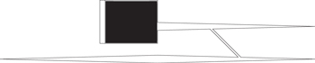
Figure 5. Initial geometry, designed to be representative of damage observed in figure 2: delamination width  and length
  . Driving pressure 1.19
  Pa.
Pa.
Download figure:
Standard image High-resolution imageThe simulations were conducted for a variety of viscosity values across the range of interest (0.001–0.3 Pa s), from which the volume of crack filled after a fixed period of time could be found. Figure 6 shows the relationship between filled volume and viscosity after 1.258 × 10⁻⁴ s, illustrating how a higher viscosity leads to a lower volume fraction filled in a fixed time. The influence of viscosity is represented here by the averaged Reynolds number, defined as  where d is the crack width at exit of the reservoir and V is an average velocity based on the volume filled at the time of measurement. Figure 7 shows a visual comparison between the fill level achieved by fluids of various viscosities at the same point in time. As the fluid passes through the constriction caused by the shear crack, differences in the fill rate between different viscosity fluids become more evident due to the constriction.

Figure 6. Volume fraction filled against Reynolds number at  1.258 × 10⁻⁴ s.
Download figure:
Standard image High-resolution image
Figure 7. Fluid position in crack for various viscosities at the same time.
Download figure:
Standard image High-resolution imageThe evolution of the free surface is also of interest. As figure 8 shows, surface tension effects produce a curved meniscus-type surface across the channel. For low values of viscosity interactions can appear between the upper and lower walls of the channel, leading in some cases to columns of resin forming over the channel as seen in figure 9. Here, due to the low viscosity of the modelled fluid, the fluid exits the shear crack in a jet like formation and preferentially fills the right side of the delamination before the left side. Once the right side is filled the increased fluid velocity into the left side causes surface waves, some of which are large enough to bridge the gap between the surfaces of the delamination (figure 9(f)) where the fluid remains due to surface tension. The momentum of the fluid then causes it to continue to travel along both surfaces at approximately the same speed.
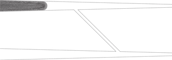
Figure 8. Flow in crack forming a meniscus under the influence of surface tension.
Download figure:
Standard image High-resolution image
Figure 9. Behaviour of 0.001 Pa s fluid exiting shear crack.
Download figure:
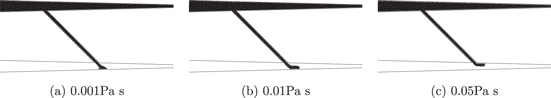
Standard image High-resolution imageAs the resin may at any time, dependant on hardening, become so viscous that further crack filling will not occur it is useful to observe how the resin exits the shear crack. If the resin does not bridge the gap between the upper and lower surfaces of the bottom delamination then the resin cannot add strength in that region. Figure 10 shows the shear crack exit behaviour for a range of viscosities. The behaviour is essentially determined by the ratio of inertial to surface tension forces; at low viscosities the fluid leaves the crack with sufficient velocity to bridge across the delamination while at higher viscosities the velocity is lower and so the surface tension keeps the fluid adhering to the upper surface of the delamination.
Figure 10. Resin behaviour exiting the shear crack.
Download figure:
Standard image High-resolution image
5. Conclusions and future work
An SPH code has been produced that is suitable for modelling the discharge of healing agent from a vascular network in self-healing composites. Here it is shown that the numerical model matches the experimental data presented by Kiljański [43] and to a closer extent that of Dziubiński and Marcinkowski [42]. With a high resolution particle distribution the limiting value of the discharge coefficient at high Reynolds numbers is matched, as is the curve fit of the coefficient of discharge as a function of Reynolds number.
An illustrative crack geometry is shown with two delaminations and a shear crack joining the delaminations; a typical damage scenario found in fibre reinforced composite materials. However, the model is not limited to this geometry, and could be readily extended to consider the ability of gap-filling scaffolds to restore large scale puncture sites in either composite materials or brittle polymeric systems [44]. The results in this paper have shown that the dependency of crack fill rate upon healing resin viscosity can be found using this model and that the small scale features such as preferential surface wetting and resin flow can be studied, leading to a greater understanding of final healed material strength.
This type of modelling opens a range of possibilities for understanding and designing vascular networks. For example, although only a single nozzle is considered here, the method readily extends to networks comprising many junctions and nozzles. It also offers the opportunity to explore a range of nozzle designs, together with the option of incorporating a variety of healing agent curing laws.
Acknowledgments
This work was carried out using the computational facilities of the Advanced Computing Research Centre, University of Bristol—http://bris.ac.uk/acrc/.