

Abstract
Since quantum-dot (QD) nanostructures in many applications are subjected to cyclic electrical and thermal loads, it is very important to analyze such nanostructures under transient thermal loads that affect the induced strains which in turn affects the response of the QD system. When the dimensions of the QDs are of the same order of magnitude as the material length scale, gradient elasticity theory should be used to account for the size-dependent behavior of such nano-sized QDs. In this work, a new finite element formulation for gradient-based thermo-electro-mechanical three-dimensional model of strained QDs in piezoelectric matrix under both static and dynamic thermal loads is developed. The proposed formulation requires only C0 shape functions since the original fourth order partial differential equation (PDE) is split into two PDEs of lower order. A unit cell of Indium Arsenide QD in a finite sized Gallium Arsenide (GaAs) substrate is analyzed. Results under dynamic loads demonstrate that the magnitude of the strain component in the thermal loading direction increases significantly with the thermal shock time. On the other hand, at a fixed time, the magnitude of the induced field quantities, such as the strain, decreases remarkably with increasing the size effect parameter. Given that large lattice mismatch induced strain fields are located in or near the QD regions, these newly observed features need to be carefully considered when designing such QD nanostructures.
Export citation and abstract BibTeX RIS
1. Introduction
Lattice mismatch or thermal expansion difference between a burried quantum-dot (QD) and a surrounding piezoelectric matrix induces both elastic and electric fields in the structure. Since both the elastic and electric fields are equally important to the understanding of the photonic and electronic features in nanostructured semiconductors [1], a reliable analysis of these fields are crucial to the design and fabrication of such structures. Several quantum mechanical methods for modifying the material optical properties were discussed in [2]. In many previous papers, semicoupled computational approaches were applied to analyze QD systems. The initial strains are computed first based on the elasticity equations. Then the purely elastic solution is used to derive the governing equations for the electric potential and electric field. Finally, the electric field is solved under suitable purely electric boundary conditions. The semicoupled approach was applied very frequently for its simplicity [3–9], but later Pan [10, 11] made a comparison between fully coupled and semicoupled models, and demonstrated that the semicoupled model could produce very serious errors for both the elastic and electric fields. Therefore, the fully coupled approach should always be used to model QD systems where piezoelectric semiconductor inclusions are embedded in a piezoelectric matrix.
Analytical solutions for an inclusion of a polygonal shape was presented in [12, 13] using the special conformal mapping method. However, conformal mapping method is inefficient for the general polygonal shape since the conformal mapping function may involve infinite terms. Green's function method [14–16] proved to be more efficient, particularly suited for polygonal shapes. The perturbation method [17, 18] also allows considering material anisotropy and arbitrary shape of inclusion. A misfitted inclusion embedded in a finite spherical matrix was analyzed in the framework of linear piezoelectricity by Seo et al [19]. Recently, Sun et al [20] analyzed quantum wires of arbitrary polygonal cross sections with graded eigenstrain in an anisotropic piezoelectric full plane. The eigenstrain field inside the inclusion is expressed as linear functions of Cartesian coordinates. A universal and efficient analytical method was proposed by Zou and coworkers [21, 22] where the quantum wires can be of any shape and the eigenstrain can be a general polynomial function of the coordinates. Jurczak and Dluzewski [23] evaluated the effect of higher-order elastic and piezoelectric coefficients on the elastic and electric fields in III-nitride wurtzite QDs.
The shape and size of the QDs play a major role in determining the optical response of QD systems. It has been demonstrated by Liu et al [24] that the shape and the area density of the QDs can be controlled by varying the growth parameters such as the growth temperature, growth rate, annealing progress and the growth interruption. Strain and piezoelectric effects are considered as tuning parameters for optical response of semiconductor nanostructures. Coupling thermo-mechanical fields (thermal expansion coefficient) and thermo-electric fields (pyroelectric parameter) can also play a very important role in QD technology. Hence temperature can also be considered as another tuning parameter. The material composition grading factor was also used as another tuning parameter [25].
Microelectronic circuits can work at extreme thermal conditions, therefore, it is important to understand the steady state and transient effects of temperature on the optoelectronic properties. Giazotto et al [26] analyzed QDs in low temperature Peltier refrigeration, whereas Chen et al [27] considered higher temperature regime. Patil and Melnik [28] studied thermoelectromechanical effects in QDs under stationary boundary conditions and steady state thermal conditions. Thermo-piezoelectricity theory allows for modeling QDs more realistically.
The first attempt to develop a theory of thermo-piezoelectricity was done by Mindlin [29]. Later, Nowacki [30] included more physical laws into that theory. Due to the complicated coupling among the three (mechanical, electrical, thermal) fields, the theory has been applied only to very simple boundary-value problems in the beginning. Analytical methods with Fourier–Hankel transformation were successfully applied to simple problems [31, 32]. The general boundary-value problem with a complex geometry requires powerful computational tools such as the finite element method (FEM) [33–36]. In recent years, meshless formulations have also become popular due to their high adaptivity and low costs in preparation of input and output data for numerical analyses. A variety of meshless methods have been proposed and some of them were also applied to thermo-piezoelectric problems [37]. The inclusion of the thermal effects may help improve the performance characteristics of intelligent structures with distributed piezoelectric sensors and actuators [38]. Three-dimensional (3D) analysis of the coupled thermo-piezoelectro-mechanical behavior of multilayered plates was done by Vel and Batra [39] and Liew et al [40]. In many of the aforementioned studies, classical continuum mechanics proved to be accurate enough to model QD systems. This was also discussed in more details in [41].
If the dimensions of the QDs are of the same order of the material length scale, classical continuum mechanics should not be applied since it neglects the interaction of material microstructure, and the results are size-independent. The atomistic models overcome intrinsic limitations of classical elasticity. The development of multiscale approaches is preferable due to the extremely high requirements on computer memory in atomistic models. The multiscale approaches bridge atomistic and continuum subdomains. However, there are observed unphysical phenomena in multiscale approaches especially for time-dependent problems. The other alternative is to apply advanced continuum theories to account for intrinsic length scales. Advanced continuum theories can be based on the Eringen's non-local elasticity [42, 43], or Mindlin's strain-gradient elasticity [44, 45]. In the non-local theory, the stress at a reference point is a functional of strains at more points of the solid body. The higher-order strain gradients are considered in the constitutive equations of the gradient theory. The two length scales in Mindlin's theory [44] are taken equal to each other in Aifantis' theory [46–48]. This greatly simplifies further mathematical and implementational treatment. Fleck and Hutchinson [49] provided an overview of the various higher-order gradient theories.
This paper presents, for the first time, the thermo-electro-mechanical 3D analyses of QDs under transient thermal ;conditions in order to assess the thermal shock effect on the electromechanical response of the QDs in applications where cyclic thermoeletric loads are applied. The gradient theory for thermo-piezoelectricity is also applied to account for the size-dependent behavior of QDs in nano-sized piezoelectric structures. Solving this problem using the FEM requires using C1-continuous elements to guarantee the continuity of the problem variables and their derivatives at the element boundaries. In this case, the additional complexity, as compared to using C0 shape functions, is considerable. Therefore, the original fourth order partial differential equation (PDE) is split into two PDEs of lower order that require only C0 shape functions. Numerical results obtained by the present gradient formulation are compared with those obtained by the classical coupled thermo-piezoelectric theory, and the influence of the size effect parameter is discussed.
The paper is organized as follows: section 2 presents the governing equations for the gradient thermo-piezoelectricity, section 3 details the FEM formulation, and section 4 describes the COMSOL model and numerical results. Conclusions are summarized in section 5.
2. One-parameter gradient theory for thermo-electro-mechanical fields
The basic feature of a QD system is its inherent initial strain, which induces electric and elastic fields in a piezoelectric material. This initial strain is associated with the lattice mismatch. Usually the QD has almost vanishing thermal conduction and thermal expansion coefficients. In this analysis, a periodic distribution of QDs in the matrix is considered, and for the numerical simulations, a representative volume element (RVE) as illustrated in figure 1 (left) is used. This piezoelectric composite structure under thermal load can be described by the theory of thermo-piezoelectricity.

Figure 1. (left) A unit cell of QD piezoelectric structure with InAs (Indium Arsenide) cubic dot in a finite sized GaAs (gallium arsenide) substrate to simulate periodic QD array in the system, (right) FE mesh around the QD (top-down view).
Download figure:
Standard image High-resolution imageMost piezoelectric materials are also temperature sensitive, i.e. an electric charge or voltage is generated when exposed to temperature variations. This effect is called the pyroelectric effect. However, for most materials, the inverse coupling, i.e., the heat generation caused by mechanical/electric fields, is very weak. Therefore, thermo-piezoelectricity with 'one-way coupling' is considered here for the QD system [28]. While the heat generation caused by mechanical and electrical fields can be neglected, the stresses and electrical displacements can be influenced by temperature variation. The governing equations of the phenomenological theory of piezoelectric materials under thermal loads consist of Maxwell's equations, the heat conduction equation and the balance of momentum. These governing equations, which are complemented by the boundary and initial conditions, should be solved for the unknown primary field variables which are the elastic displacement vector field ui(x, τ), the electric potential ϕ(x, τ) (or, its gradient, the electric field vector Ei(x, τ)), and the temperature difference from the reference room temperature θ(x, τ), where x is the position vector and τ is the time. Taking into account the typical material coefficients, it can be found that the characteristic frequencies for thermal, elastic and electromagnetic processes are fth = 10−3 Hz, fel = 104 Hz and felm = 107 Hz, respectively. Thus, if we consider such bodies under transient loadings, with temporal changes corresponding to fth and/or fel, the changes of the electromagnetic fields can be assumed to be immediate, or in other words the electromagnetic fields can be considered quasi-static [50].
The strain tensor εij, the electric field vector Ej and the temperature gradient vector βj are related to the displacements ui, the electric potential ϕ and the temperature θ, respectively, by

The elastic strain is given by subtraction of the eigenstrain and thermal strain from the total strain
where αij is the coefficients of linear thermal expansion,  is the eigenstrain tensor and am, aQD are lattice constants of the matrix and QD, respectively. The reference state for displacements is specified by vanishing eigenstrains and at temperature θ = 0. As the substrate is relatively large compared to the QD, we follow common practice to neglect lattice mismatch inside the matrix and to assume homogeneous eigenstrains inside the QD [28].
The strain-gradient tensor is defined as

If the size of the QDs is comparable to the size of the material microstructure, the results will be size-dependent. In this case, the classical elasticity theory should be replaced by an advanced continuum theory to account for the intrinsic length scale of the material. The one-parameter gradient theory is applied to the piezoelectric solids under thermal loads in this work. The deformation energy density in gradient theory for thermo-piezoelectricity is written as [51, 52]
where cijkl, eijk, hij, pi and κij are the material elastic, piezoelectric, dielectric, pyroelectric and thermal conductivity tensors in the thermo-piezoelectric medium, respectively. The tensor gijklmn represents the purely non-local elastic effects, i.e., the elastic strain-gradient elasticity. The stress–temperature modulus γij is expressed in terms of the elastic stiffness coefficients cijkl and the linear thermal expansion coefficients αkl as γij = cijklαkl.
Under infinitesimal deformation, the Cauchy stress σij, the higher-order stress τijk, the electric displacement Di can be expressed in terms of the derivatives of the deformation energy density as


Equation (8) is the Fourier's law for thermal conduction. Note that in uncoupled thermo-elasticity, stresses are functions of temperature, but the heat flux is independent of the elastic and electrical fields. Constitutive equations (5), (7) and (8) for material with cubic symmetry can be written in matrix form, using the reduced Voigt notation, as
where
where εijr = εij − εij*.
Equations (9)–(11) can be written in compact form as
The higher-order stress tensor τijk can be written in terms of the Cauchy stress tensor giving the total stress tensor Tij in the form [48]

where l is the internal length material parameter. One can observe that in the limit, l → 0, the total stress is equal to the Cauchy stress known from the classical ('non-gradient') elasticity. In an earlier paper, the authors derived the governing equations for the gradient piezoelectricity without thermal effects [53]. The equilibrium equation for the total stress can be rewritten in terms of the Cauchy stress [54] as

where vanishing body forces are assumed. The governing equations for the electrical and thermal fields (Maxwell's and heat conduction equations), with vanishing volume density of free charges and density of heat sources, are expressed as


where ρ and c are the mass density and specific heat, respectively. Dots over a quantity indicate time derivatives. Considering that the size effect is restricted to only elastic strains, the constitutive equation (5) can be substituted into the equilibrium equation (15) to get
This is a PDE of the fourth order. If traditional finite elements are used for the numerical solution of such problems, then C1 displacement continuity is required. Askes et al [55] presented a decomposition technique, where a set of Helmholtz equations associated with the theory of gradient elasticity were solved to handle the gradient dependence. In this case, the additional complexity as compared to C0 shape functions is considerable. In the present paper such a technique is applied to gradient piezoelectricity under a thermal load. So, the original fourth order PDE (18) is split into two PDEs, (19) and (20), of lower order that require C0 shape functions in the finite element interpolation.
If we use the notation

the PDE (18) can be expressed as

The strain εijec can be expressed by the kinematic equation

The boundary conditions for the coupled equations are different from those valid for the original fourth order format of gradient elasticity [55]. The following essential and natural boundary conditions are considered for the mechanical field represented by equation (20):
where ni is the unit vector normal to the domain boundary,  are the prescribed tractions at
  boundary, which is a part of the global domain boundary, and
  are the prescribed displacements at Γu boundary. For the electrical and thermal fields, we have:

where Γp, ΓQ, Γθ, and Γq are the boundaries where electric potential  surface charge density
  temperature difference
  and heat flux
  are prescribed, respectively.
The essential and natural boundary conditions for the Helmholtz equation (19) are given by
Initial conditions for the mechanical and thermal quantities are assumed as:
In the next section, a finite element formulation is developed to analyze the above stated boundary-value problem of the gradient-based thermo-piezoelectricity.
3. Finite element formulation
The FEM is developed here for the problem described by the system of PDEs (16), (17), (19) and (20). Since uncoupled thermo-elasticity is considered, the heat conduction problem is analyzed separately and the weak/variational forms are given by

δθ is a test function such that 
The weak forms for the rest governing equations are given by

The used test functions are such that 
 and
and 
The primary field variables in the above weak forms can be approximated over each standard finite element Ve in the FEM. The fields are expressed in terms of their respective nodal values and the corresponding shape function N(a)(ξ1, ξ2, ξ3) as
where the superscripts (a) denote the global number of the ath node of Ve, (a = 1, 2, ..., n). The gradients in the Cartesian coordinate system are expressed in terms of the derivatives with respect to the intrinsic coordinates as
Hence,
and 
It is convenient to introduce the following column vectors:
where  The approximations of the secondary fields on Ve can now be written as:

To simplify the FEM equations further, we consider vanishing pyroelectric coefficient. The variations of the primary field variables can be also expressed in terms of the variations of the nodal values. Thus, the variational statements, (27)–(29), can be rewritten as
where C, L and A are matrices of elastic, piezoelectric and dielectric constants, respectively. Since the variational forms (40)–(43) are, respectively, valid for any arbitrary δθa, δϕa, δuc(a) and δεa satisfying the Dirichlet boundary conditions, the following system of ordinary differential equations and algebraic equations is obtained:
where ek denotes the finite element  involving the node xk, and ak is the local number of the node xk on
4. Numerical results
For a periodic distribution of QDs in a 3D piezoelectric matrix we consider a RVE with prescribed temperature on its upper surface (figure 1 (left)). The RVE is assumed to have a cubic geometry with side length of 40 nm, and a cubic QD with side length of a = 4 nm is embedded in it. The top surface of the InAs QD is 4 nm from the top surface of the matrix. Material properties of the InAs dot are [56]
Matrix (substrate) is made of GaAs, whose properties are
It follows from the lattice constants that the eigenstrains are  The pyroelectric coefficient p1 is not considered in the numerical analyses since this quantity is small and would have only very small influence on the results.
The four side faces of the matrix are fixed along their normal direction, the bottom face is fixed along its normal direction, and the upper surface is free of tractions. Lateral sides and bottom side of the matrix cube are thermally isolated. Temperature is prescribed on the top. All surfaces have vanishing normal component of electric displacement, except for the bottom side, where a vanishing electric potential is prescribed. Then, one can write the following boundary conditions for the InAs/GaAs electronic structure (figure 1 (left)):
On surfaces BCGF and ADHE: u1 = 0, t2 = t3 = 0, D1 = 0, q = 0;
ABFE and DCGH: u2 = 0, t1 = t3 = 0, D2 = 0, q = 0;
ABCD: u3 = 0, t1 = t2 = 0, ϕ = 0, q = 0;
EFGH: t3 = 0, t1 = t2 = 0, D3 = 0, θ = θ0.
On the interface between InAs and GaAs, the continuity of displacements, electric potential and temperature has to be satisfied, namely,

as well as the reciprocity of traction vector, electric displacement and heat flux
Vanishing natural boundary conditions for the Helmholtz equation (19) are considered on all surfaces (see equation (25)).
A 3D COMSOL model was created by constructing the geometry and meshing it using 195 696 SOLID elements corresponding to 339 117 nodes as shown in figure 1 (right). COMSOL Multiphysics allows for implementing the governing equations (27)–(29) in the Weak-Form module. Computer code results were verified by ANSYS when the structural material parameter is vanishing (classical theory).
Majdoub et al [57] published material parameters for the enhanced size-dependent piezoelectricity and elasticity in nanostructures, and it follows that l = 0.5 × 10⁻⁹ m. However, in our numerical analyses we considered various values of the intrinsic material characteristic (size effect parameter), l, to illustrate its influence on strains. This material parameter represents micro-structural size, and therefore it has to be smaller than the size of the QD, a. As such, the admissible dimensionless ratio l/a should be restricted to the range from 0 to 1.
4.1. Code validation
In this section, numerical results obtained using COMSOL are compared with the ones obtained by ANSYS for classical theory, l = 0. For comparison, we have selected the applied thermal load to be 500 °C. The variation of the strain component ε11 along X1-direction (passing the QD center) and electric potential ϕ along X3 (aligned with the edge of the QD at X1 = 18 nm and X2 = 22 nm) is presented in figure 2. One can observe excellent agreement between COMSOL and ANSYS results with error less than 1% for both the strain and electric potential.

Figure 2. Elastic strain component ε11 along X1-direction (passing the QC center) (upper) and the potentials ϕ along X3 at X1 = 18 nm and X2 = 22 nm (bottom) using COMSOL and ANSYS.
Download figure:
Standard image High-resolution image4.2. Static analysis of cubic QD in a cubic matrix
The electric potential contour plots in the X1X2- and X2X3-planes are shown in figure 3 where the prescribed temperature on the top surface of the matrix is 250 °C under stationary conditions. Electric potential on the X1X2 plane with X3 = 32 nm is similar to that in figure 3 (bottom). Figure 4 shows the contour plots of the electric field intensity EX1 at X1X2- , X1X3- and X2X3-planes.

Figure 3. Electric potential contours ϕ (V) on the (upper) X1X2-plane with X3 = 32 nm, (bottom) X2X3-plane with X1 = 18 nm.
Download figure:
Standard image High-resolution image
Figure 4. Electric field intensity EX1 (V m−1) on the (upper) X1X2-plane with X3 = 32 nm, (middle) X2X3-plane with X1 = 18 nm, (bottom) X1X3-plane with X2 = 18 nm.
Download figure:
Standard image High-resolution imageIt can be observed from figure 3 that due to the cubic symmetry and the fact that the QD center is away from the top surface, the electric potential distributions on the X1X2- and X2X3-planes are very similar. The highest concentration of the electric potential is near the corners of the QD cube and is anti-symmetric. However, the electric field intensity, which is the derivative of the electric potential, on the corresponding planes is substantially different. This is demonstrated clearly in figure 4 for the electric field intensity EX1 at X1X2- , X2X3- and X1X3-planes where one can observe field concentrations at the four corners on the X1X2- and X1X3-planes but not on the X2X3-plane. This strange feature is due to the fact that in the first two cases the electric field intensity EX1 is obtained by taking the derivative of the potential with respect to X1, which is within these planes, whilst for the last case (in the X2X3-plane), the derivative is out of plane.
Contour plots for strain components ε33 and ε12 on the X1X2-plane with X3 = 34 nm are presented in figure 5. It is clearly observed that while the normal strain is concentrated within the QD region, the shear strains show field concentration at the corners.

Figure 5. Strain component (upper) ε33 and (lower) ε12 on the X1X2-plane with X3 = 34 nm.
Download figure:
Standard image High-resolution imageNext, the influence of temperature prescribed on the upper surface of the QD electronic structure EFGH in figure 1 is investigated. Figures 6 and 7 show the variations of total normal strains along the X1- and X3-directions, respectively, passing the QD center (X1 = X2 = 20 nm, X3 = 34 nm) at various temperatures 0 °C, 250 °C, and 500 °C with classical elasticity (l = 0) (left) and gradient elasticity (l = 5 × 10⁻¹⁰) (right). It can be seen that the effect of temperature on the electromechanical quantities of GaAs/InAS QD system is not significant. A similar phenomenon was observed by Patil and Melnik [28] for cylindrical GaN/AlN QDs. The magnitude of all strain components decreases with increasing distance away from the QD. When l increases, the effect of temperature on strains increases as can be seen in figure 7. Under a given temperature, however, the magnitude of these normal strains can be significantly decreased with increasing material parameter length l, which is further demonstrated in figure 8.

Figure 6. Distribution of total normal strain ε11 in the X1-direction passing the QD center at various temperatures with (left) classic elasticity (l = 0), (right) gradient elasticity and specific size effect parameter.
Download figure:
Standard image High-resolution image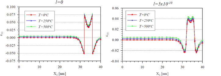
Figure 7. Distribution of total normal strain ε33 along X3-direction passing the QD center at various temperatures with (left) classic elasticity (l = 0), (right) gradient elasticity and specific size effect parameter.
Download figure:
Standard image High-resolution image
Figure 8. Distribution of total normal strain (upper left) ε11 along X1-direction, (upper right) ε33 along X3-direction (passing the QD center), with various size effect parameter l at constant temperature, and (lower) the variation of the maximum strain ε11 with increasing l/a ratio.
Download figure:
Standard image High-resolution imageFigure 8 (upper left and right) shows the influence of the material characteristic length, l, on the normal strains ε11 and ε33 in figures 6 and 7 at a constant temperature (250 °C). As the size effect parameter, l, increases, the magnitude of the strains decreases significantly and therefore the corresponding system becomes stiffer. Figure 8 (lower) illustrates the variation of the maximum strain ε11 with l/a ratio. As the QD size gets smaller with respect to the parameter l, the strains decrease. This provides a new opportunity for designing stiffer QD nanostructure by decreasing the size of the QDs to the level that experiences this size effect. Furthermore, size effect eliminates the sharp transitions of the strains at the interfaces of the boundaries, reducing the field concentration, and thus making the structure safer.
4.3. Transient analysis
To consider a transient thermal load, a 500 °C temperature shock load on the upper surface of the matrix is prescribed. The variations of strain components ε11 and ε33 along the X1- and X3-directions, respectively, are presented in figures 9 and 10. The line l = 0 corresponds to classical elasticity at time τ, under thermal shock load with τ = 7 × 10⁻¹³ s. Figure 11 shows the time evolution of maximum strains ε11 and ε33 at l = 5 × 10⁻¹⁰. Although steady state temperature proved to be insignificant on the strain distribution of the QD system, as was shown in section 4.2, when the system is subjected to transient or cyclic thermal loads, the induced strains vary substantially with time. On the other hand, increasing the size effect parameter is always stiffening the system and reducing the induced strains. These trends need to be carefully considered when the nanostructure is under thermal dynamic loads.

Figure 9. The variation of total strain component ε11 along the X1-direction (passing the QD center) under thermal shock load (left) at τ = 7 × 10⁻¹³ s and two size effect parameter, (right) with l = 5 × 10⁻¹⁰ and increasing time.
Download figure:
Standard image High-resolution image
Figure 10. The variation of total strain component ε33 along X3-direction (passing the QD center) under thermal shock load (left) at τ = 7 × 10⁻¹³ s and two size effect parameter, (right) l = 5 × 10⁻¹⁰ with increasing time.
Download figure:
Standard image High-resolution image
Figure 11. The evolution of maximum strain (left) ε11, (right) ε33, with time τ [s].
Download figure:
Standard image High-resolution image
5. Conclusions
To assess the effect of a thermal shock load on a QD embedded in a piezoelectric substrate, a 3D dynamic thermo-piezoelectric finite element model has been developed. The model is a RVE that is used to simulate periodic QD array in the system and analyze the gradient elastic and piezoelectric fields induced by stationary and transient thermal loads. It was observed that the largest magnitudes of the induced field quantities, such as the induced strain fields, are within or near the QD regions, indicating that the effect of the lattice mismatch dominates. It was also found that as the size of QDs in the system gets smaller, the size effect parameter makes the system stiffer and reduces the induced strains. In addition, dynamic thermal loads proved to have a significant effect on the induced strains and the QD overall performance. Accordingly, the reported observations should be considered when designing strained QD nanostructures subjected to cyclic electrical and thermal loads.
Acknowledgments
The authors gratefully acknowledge the supports by the Slovak Science and Technology Assistance Agency APVV-14-0216 and the Slovak Grant Agency VEGA-1/0145/17.