
Abstract
We present a systematic implementation of the recently developed Z-method for computing melting points of solids, augmented by a Bayesian analysis of the data obtained from molecular dynamics simulations. The use of Bayesian inference allows us to extract valuable information from limited data, reducing the computational cost of drawing the isochoric curve. From this Bayesian Z-method we obtain posterior distributions for the melting temperature Tm, the critical superheating temperature TLS and the slopes dT/dE of the liquid and solid phases. The method therefore gives full quantification of the errors in the prediction of the melting point. This procedure is applied to the estimation of the melting point of Ti2GaN (one of the so-called MAX phases), a complex, laminar material, by density functional theory molecular dynamics, finding an estimate Tm of 2591.61 ± 89.61 K, which is in good agreement with melting points of similar ceramics.
1. Introduction
The problem of determination of thermodynamical properties of complex materials via computer simulation is a challenge for computational materials science. In particular, determination of melting points of complex substances involves long, expensive first-principles molecular dynamics (MD) simulations, and in this respect, an efficient procedure to compute Tm from as few independent simulations as possible would be highly desirable [1]. In this work, we approach this issue from the point of view of Bayesian statistics, a methodology based on the computation of probabilities for the unknown parameters of a problem [2, 3]. We develop a Bayesian version of the recently proposed Z-method [4], in which energy–temperature points (E, T(E)) obtained from a microcanonical simulation are post-processed to infer the most probable Tm and TLS together with their respective uncertainties. We apply this new methodology to the computation of the melting point of Ti2GaN, an interesting ceramic-like material, which as far as we know has yet to be measured experimentally.
Ti2GaN is a complex, layered ternary compound which belongs to the so-called MAX phases. In the search for new structural materials for use in the aerospace, automotive and chemical industries, MAX phases are gaining importance due to their remarkable combination of properties, somewhere in between metals and ceramics (i.e. stiff, lightweight and ductile) [5–7]. MAX phases are made up of an early transition metal M, an element A from the III-A or IV-A group of the periodic table, e.g. Ga or Ge, and X which is either C or N, in the composition Mn+1AXn, where n is 1, 2 or 3. The technological interest comes from their mechanical and resistance properties, as they have the thermal and electrical conductivities of metals but the elastic rigidity of ceramics. Like metals, they present good electrical and thermal conductivities ranging from 0.5 to 14 × 106 Ω−1 m−1, and from 10 to 40 W m−1 K−1, respectively, and are relatively soft, having Vickers hardness of about 2–5 GPa. Like ceramics, they are elastically stiff, and some of them, e.g. Ti3SiC2, Ti3AlC2 and Ti4AlN3, also exhibit excellent high-temperature mechanical properties. They are resistant to thermal shock and unusually damage-tolerant, and exhibit excellent corrosion resistance. Moreover, unlike conventional carbides or nitrides, they can be machined by conventional tools without any lubricant, which is of great technological importance for applications. The need for thermodynamic and thermophysical data as well as an atomic level understanding of their properties cannot be overemphasized.
There are, however, scarce experimental measurements and theoretical predictions for the vast majority of these materials, in particular at high temperatures. For example, even for Ti3SiC2, the most studied of the MAX phases, which is resistant to oxidation and thermal shock and capable of remaining strong up to temperature in excess of 1300 °C in air, its structural stability above 1400 °C remains unclear [8]. The same lack of information exists about the melting curve of these materials. Thus, it would be desirable to have reliable high-temperature information in order to anticipate further applications.
In this paper we chose a particular example among the MAX phases, namely Ti2GaN, to show how the melting point can be calculated using a state-of-the-art computer simulation methodology. Recently, ab initio static calculations have been performed in order to predict their structural and elastic properties [9]. But also ab initio MD calculations should make it possible to predict other, more complex properties, such as diffusion coefficients and the melting curve.
The rest of the paper is organized as follows. In section 2, we describe the methodology for the estimation of the melting curve by computer simulation. Section 2 also presents the statistical analysis used, based on Bayesian statistics. The results, as well as the details of the ab initio calculation, are presented in section 3. Finally, in section 4 we draw the main conclusions of our work.
2. Methodology for computing melting points
In spite of being one of the most ubiquitous and everyday phenomena, a physical explanation of the nature of melting is still lacking. In the same way, there is no analytical expression which allows one to predict the melting point of a material. So far, the most popular approach to estimate the melting point is via computer simulation. Several different methods have been devised to do so, among them: free energy perturbation [10], thermodynamic integration [11–13] and the two-phase method [14]. A relatively recent approach to determine the melting point using MD is the Z-method [4, 15–18], which is a microcanonical one-phase method based on the superheating effect.
2.1. The Z-method
In microcanonical MD simulation it has been found empirically that, when starting from the ideal crystalline structure and increasing the total energy at a fixed volume V, there is a well-defined maximum (for the solid phase), ES(TLS; V) where TLS corresponds to the limit of the superheating temperature. Increasing the energy beyond ES by a small amount δE, the solid spontaneously melts at ES + δE ≈ ES, but due to the increase in potential energy, namely the latent heat of fusion, the temperature decreases. The interesting fact is that the final temperature after melting at ES seems to coincide with the melting point Tm obtained from other methods. Thus, the following equivalence is established in practice.

The procedure for the Z-method computation of the melting point is then as follows: at a fixed volume, the (E, 〈T〉) points (where 〈·〉 means average) from different simulations draw a 'Z' shape, as shown in figure 1(a), hence the name of the method. Note that one also can draw the isochore in the pressure–temperature plane (〈p〉, 〈T〉), as is shown in figure 1(b). In these Z-shaped curves the sharp inflection at the higher temperature corresponds to TLS and the one at the lower temperature to Tm. Thus, knowledge of the lower inflection point for different densities allows the determination of the melting curve for a particular range of pressures.
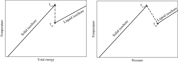
Figure 1. Schematic representation of the isochoric lines in Z-method simulations. (a) energy–temperature plane; (b) pressure–temperature plane.
Download figure:
Standard image High-resolution imageFrom figure 1 it can be seen that finding the intersection between the solid and liquid isochores constitutes a lower bound for Tm. Moreover, as TLS − Tm becomes smaller (pressures near zero), this lower estimate moves closer to Tm, thus finding the temperature at which the isochoric line changes slope can be a reasonable estimate of Tm. However, we can do better by taking advantage of the full set of points in a Bayesian estimation of the parameters defining the Z-curve, namely TLS, Tm, ELS and the slopes of the solid and liquid branches, related to the heat capacities of the solid and liquid phases, CS and CL, respectively.
2.2. Bayesian probability
The Bayesian school of statistics [2, 3] extends 'classical' (or 'frequentist') probabilities, which are defined as frequencies in repeatable experiments and only applicable to random variables, to any proposition that can be said to be true or false, including allowed values of unknown (but not random) parameters. Thus Bayesian probabilities are expressions of human ignorance about the truth of some arbitrary proposition (for instance, asserting the correct value of a parameter) rather than immutable properties of random variables. Bayesian probabilities can (and should) be updated under new information, and that is where Bayes' theorem enters. It connects the probability of a certain hypothesis H under study, before and after the acquisition of new evidence. This connection is made by means of the likelihood function, which is the probability of observing the evidence if our hypothesis is indeed true. Formally,

where H is the hypothesis to be tested, E is some evidence relevant to H, I0 represents our initial (or prior) state of knowledge, that is before including E, and the notation P(α|β) represents the probability of proposition α being true, given that proposition β is true. Here P(H|I0) is the prior probability of H, P(H|E) is the posterior probability of H, and P(E|H) is the likelihood function. P(E|I0) is the prior probability of the evidence (often referred to as simply the evidence), and is usually treated as a normalization constant.
Suppose Hk asserts that the unknown parameter x ∈ {x1, ..., xN} takes the value xk. We can simply denote Hk by xk and then Bayes' theorem reads

where we have determined P(E|I0) from the normalization condition

Equation (3) gives us the posterior distribution for the parameter x, which allows us to assert which regions of the parameter x we believe are the most probable given the evidence E. Thus, it is a summary of our knowledge of the parameter after incorporating the evidence E. In section 3 it will be shown how this approach is applied to the melting problem.
2.3. Ab initio MD simulations
An initially crystalline structure of Ti2GaN (symmetry group P63/mmc) was prepared, consisting of 96 atoms (48 Ti, 24 Ga and 24 N) and 2 × 2 × 3 unit cells. The lattice parameters a0 = 3.018 Å and c0 = 13.318 Å were taken from first-principles calculations by Bouhemadou [9]. The final lengths of the simulation cell were then a = 6.036 Å, and c = 39.954 Å. This structure was subjected to an ionic relaxation procedure using VASP [19], the resulting structure is shown in figure 2, left panel. After that, we proceed with the MD runs at different total energies E.

Figure 2. Left, initial crystalline structure of Ti2GaN; right, liquid structure.
Download figure:
Standard image High-resolution imageAll MD calculations were performed using density functional theory (DFT) as implemented in the VASP code. Perdew–Burke–Ernzerhof (PBE) generalized gradient approximation (GGA) pseudopotentials [20] were used, with an energy cutoff Ec = 300 eV and the valence wavefunctions expanded at the Γ point. The time step used for the Born–Oppenheimer MD was 1 fs.
3. Results
Z-method simulations were performed on the above described 96-atom Ti2GaN system, for at least 2.5 ps at each simulated energy, and averages were taken over the last 0.5 ps. The results are shown in figure 3. This plot, in practice, has been obtained as follows: working in the microcanonical ensemble (E, V, N), we start by assigning a given kinetic energy to the ideal crystalline structure, corresponding to a total energy E. After a while, following the equipartition theorem, the system equilibrates, reaching a temperature T(E) (which is usually around half the initial temperature). If, after a long simulation time (typically hundreds of picoseconds) the system still remains at the average temperature T, then it is in the solid phase (as shown by the asterisks at E < −60 eV/unit cell in figure 3). If the final average temperature is lower, then the system melts: the lattice becomes disordered, increasing the potential energy and therefore decreasing the temperature (asterisks at E > −60 eV/unit cell in figure 3).

Figure 3. Isochoric curve for Ti2GaN as determined from DFT-MD simulations. The decrease in temperature around E = −59.92 eV/unit cell signals the melting point. Inset shows the region around E = −59.92 eV/unit cell, and the error bars correspond to the uncertainties in TLS (upper) and Tm (lower) computed by the Bayesian procedure.
Download figure:
Standard image High-resolution imageFigure 4 shows the radial distribution function (RDF) g(r) for Ti–Ga pairs and the species-weighted, or total, g(r). The g(r) function for Ti–Ga shows a qualitative change on melting (the double-peak structure around 4.3 Å is lost in the liquid), and the total g(r) shows clearly there are atoms in between the original solid layers (2.4 and 3.3 Å).

Figure 4. RDFs for Ti–Ga pairs (upper panel) and all pairs (lower panel) for both liquid (T ≈ 4000 K) and solid (T ≈ 1000 K) phases.
Download figure:
Standard image High-resolution imageIn order to extract the most information out of the limited number of points (especially on the region near ELS) and the considerable fluctuations of temperature in the liquid branch, we developed a Bayesian analysis technique [3] to produce estimations for all the parameters involved in drawing a Z-curve. Because the novelty of our procedure to obtain the melting point is not in the Z-method itself, but in the analysis of its results by the Bayesian approach, we will explain it in detail.
The relevant parameters involved in the drawing of the Z-curve are Tm, TLS, and the slopes of the solid branch (1/CS) and the liquid branch (1/CS). These four parameters are sufficient as the superheating energy ELS is completely fixed by knowing TLS and CS, by means of the relation

where Φ0 is the potential energy of the initial ideal structure, which is known in advance exactly. We then construct the posterior distribution P(Z|{Di}) where Z represents the four-tuple Z = (TLS, Tm, CS, CL) and {Di} is a set of measured points Di = (Ei, Ti) obtained from the MD simulation. These are the points one usually joins 'by hand' to draw the best Z-curve. In order to obtain the posterior distribution, and therefore, what are the best parameters Z as suggested by our measured points, we need the likelihood function P ({Di}|Z), that is, the probability of measuring these points exactly given a hypothetical set of parameters Z. For this, we need to make some assumptions about the measurement errors.
We assume normally distributed errors for the measurements of both E and T, with standard deviations σE and σT, respectively. Despite the simulations being microcanonical, there is a small (compared with the fluctuations in temperature) numerical error in the total energy, which is taken as σE.
As both axes T and E now are subject to experimental error, the usual least-squares procedure is not strictly valid [21]. In order to construct the likelihood function for the data points, we write the probability of measuring a single point Di given that the real point belongs to the solid branch (S), liquid branch (L), or is a mixed point (M), that is, a point for which melting happened during the 'averaging' phase of the simulation, thus resulting in a temperature in between Tm and TLS. For the case of the solid branch, we have


where

is the normal distribution and the notation P(Di|Z, bi = S) should be read as the probability of observing the ith point given that the Z-curve parameters are Z and the ith point belongs to the solid branch. Similarly, for the case of the liquid branch,

For both cases (solid and liquid branches), the probability of measuring Di if the corresponding real point belongs to a specific branch (denoted by b) is given, after integration and proper normalization, by the form


where

is the cumulative distribution function (CDF) for the normal distribution, and the following definitions were made for simplicity of notation.


In defining these quantities we have let, for the solid branch, C' = CS, E' = Φ0 and T' = TLS, whereas for the liquid branch C' = CL, E' = ELS and T' = Tmax − Tm.
Finally, for the case of a mixed point,

which reduces, after integration and normalization, to

We used simple, flat priors for the parameters, just imposing the consistency conditions for them to represent a valid Z-curve, namely


which, when considered together, lead to the full prior

where Θ(·) is the Heaviside function, is the highest measured point of the solid branch (minus three standard deviations in both axes to account for the measurement error) and is the lowest measured point of the liquid branch (plus three standard deviations in both axes). That is, these points are taken from the data as a lower bound for (ELS, TLS) and a higher bound for (Em, Tm), respectively. Note that we are using just the extreme values from the data to construct the prior, but these extreme values could come from other sources (for instance empirical data, thermodynamic considerations and so on). So, this is not an uninformative prior, however any redundancy between the information included in the prior and the one included in the likelihood function cannot distort the inference process [22].


Application of Bayes theorem (equation (2)) then gives the posterior distribution for the four-tuple Z,

where bi is the corresponding branch for the ith point (one of S, L, M), which we can determine by simple inspection of the instantaneous temperature or the dynamical properties of the final sample. The posterior distribution for each of the parameters, shown in figures 5–9 was sampled numerically via a Metropolis–Hastings Monte Carlo (MC) algorithm [23] and histograms were collected during 2 × 10⁵ MC steps (see tables 1 and 2).

Figure 5. Posterior distribution for the melting temperature P(Tm|{Di}) as obtained from the DFT-MD simulations.
Download figure:
Standard image High-resolution image
Figure 6. Posterior distribution for the critical superheating temperature P(TLS|{Di}) as obtained from the DFT-MD simulations.
Download figure:
Standard image High-resolution image
Figure 7. Posterior distribution for the superheating energy P(ELS|{Di}) as obtained from the DFT-MD simulations.
Download figure:
Standard image High-resolution image
Figure 8. Posterior distribution for the solid heat capacity P(CS|{Di}) as obtained from the DFT-MD simulations.
Download figure:
Standard image High-resolution image
Figure 9. Posterior distribution for the liquid heat capacity P(CL|{Di}) as obtained from the DFT-MD simulations.
Download figure:
Standard image High-resolution image
Table 1. Interval estimations obtained from the posterior distributions for TLS, Tm and ELS. The error bar has a width of one standard deviation (approximately 68% confidence).
| Tm (K) | TLS (K) | ELS (eV/unit cell) |
|---|---|---|
| 2591.91 ± 89.61 | 2721.87 ± 57.32 | −59.94 ± 0.01 |
Table 2. Interval estimations obtained from the posterior distributions for CS and CL. The error bar has a width of one standard deviation (approximately 68% confidence).
| CS (kB/atom) | CL (kB/atom) |
|---|---|
| 3.02 ± 0.06 | 3.05 ± 0.53 |
The calculated posterior estimate for the melting point is Tm = 2591.91 ± 89.61 K, which is close to values found in ultra-high-temperature ceramic (UHTC) composites [24], for instance, SrZrO3 with 2327 K, TiN with 2677 K, TiC with 2827 K and TiB2 with 2952 K.
Quite purposely we have not dealt with corrections to the Z-method due to the limited number of atoms or time steps in the simulation, which for small systems could be the largest contributions to error. The Bayesian procedure described here is intended as a complementary tool once corrections to finite-size and finite-time effects are in place. It is well known [15, 25] that increasing the duration of each MD simulation should decrease the obtained values of both TLS and Tm, and in this sense, every Z-method estimation of Tm should be taken as an upper bound for the 'real' Tm (in the thermodynamic limit and for infinite simulation time). These limitations can also be present in two-phase simulations, and they should be dealt with by extrapolation using different sizes and simulation times (if possible, according to computational requirements). Although this calculation is then a preliminary estimation, this result is the first (to the best of our knowledge) prediction of the melting point for this complex ceramic, and it can be useful as a hint for a 'search space' to explore in future Z-method simulations with larger sizes and simulation times.
4. Concluding remarks
We have obtained an estimation for the melting point of Ti2GaN, a complex material belonging to the so-called MAX phases, by means of first-principles microcanonical one-phase simulations (the recently developed Z-method), improved with a novel Bayesian methodology to infer the parameters of the Z-curve (together with their uncertainties) from molecular dynamics data. The melting point thus obtained agrees quite well with those of other traditional, high-temperature ceramics, around 2600 K, particularly close to TiN with 2677 K.
The Bayesian Z-method proposed here should be applicable (and especially suited) to systems under non-negligible thermodynamic fluctuations, which is the case for ab initio simulations with under a hundred atoms.
Acknowledgments
This work was funded by FONDECYT 3110017. GG acknowledges project ENL 10/06 VRID-Univ. de Chile and partial support from FONDECYT 1120603.