
Abstract
A frame indifferent formulation of the energy and force on a dislocation in a line tension model in an anisotropic elasticity media is presented. This formulation is valid for any dislocation line direction and Burgers' vector and expresses the energy and force in terms of an integral for which no general analytical solution can be calculated. Three numerical methods are investigated to evaluate the energy and the force: direct numerical integration, spherical harmonics expansions and an interpolation table method. We analyze the convergence and computational cost of each method and compare them with a view to selecting the most appropriate for implementation in large scale dislocation dynamics codes.
Export citation and abstract BibTeX RIS
1. Introduction
Some dislocation interactions, e.g. bow-out, cross-slip and junction formation, are well captured by computing only an approximation of the total force on the dislocation. This approximation, the orientation-dependent line tension model, represents dislocations as flexible strings. It assumes a simple energy per unit length of dislocation line and neglects the interactions between dislocations. It has been used to compute the critical stress at which a dislocation bows out [1] and to determine the shape of a dislocation glide loop at equilibrium [2] for general anisotropy. It has also proven effective in determining binary dislocation interactions as a function of their angle of incidence [3–7].
Line tension expressions for the force and the energy in anisotropic elasticity have been derived by Bacon et al in [8]. In sections 2 and 4 respectively, we revisit the formulation of energy and force in the line tension approximation and rewrite the expressions in a coordinate-independent form. The formulation proposed by Bacon et al [8] is extended to all Burgers' vectors and line directions instead of being defined only in the plane containing the line direction of the dislocation and its Burgers' vector.
The cost of computing energy in the line tension model is not negligible. A comparison is made between three methods of evaluating the energy and the force: a direct numerical integration method (section 3.1); a spherical harmonics expansion (section 3.2); and an interpolation table method (section 3.3). We study the cost and accuracy of each method as a function of the anisotropy ratio (defined as A = 2C44/(C11 − C12) in cubic crystals where C11, C12 and C44 are the elastic constants; A = 1 for an isotropic material) to determine which one is most suitable for implementation in large scale dislocation dynamics codes.
2. Energy in anisotropic elasticity
The strain energy per unit length of dislocation line in anisotropic elasticity is given in Bacon et al [8] by

where R and a are the outer and inner cut-off radii, and E is the pre-logarithmic energy factor given by

E is uniquely determined by the Burgers' vector b of the dislocation line, and the 3 × 3 matrix B(t) given by

where the unit vectors m and n are orthogonal to t, the dislocation line direction. The notation (mm) is such that (mm)jk = miCijklml where Cijkl is the fourth order elasticity tensor.
Similarly to Bacon et al [8], the two orthogonal unit vectors m and n can be defined by

where ω is the integration variable. It varies in [0, π] (see figure 1).
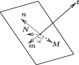
Figure 1. Notation for energy and force formula in anisotropic elasticity. t is the line direction, (M, N) are two unit vectors orthogonal to t and (m, n) are two unit vectors rotating around (M, N) with an angle ω and orthogonal to t.
Download figure:
Standard image High-resolution imageN is defined as the normalized vector

where the matrix D is such that D ≡ I − t ⊗ t, where I is the identity matrix, the rows of D correspond to a set of vectors orthogonal to t. Define α as the index for which the component j of the vector v defined as
is maximum. Dα = (Diα)i=1,2,3 is one non-vanishing vector orthogonal to t that can always be defined.
Defining M = N × t, we have two unit vectors (M, N) orthogonal to t that are well defined for all orientations. By construction, (t, M, N) form an orthonormal basis independent of the Burgers' vector b.
In Bacon et al [8], equation (3) and its derivatives are given as angular derivatives of the line direction t with respect to an angle between the line direction t and some arbitrary fixed direction. In definitions (4)–(6), the fixed direction is Dα and it depends on t which allows M, N, m and n to always be well defined.
3. Methods to compute the energy
The complexity of calculating the energy
 , equation (1), resides in the definition of the matrix B, equation (3). Aside from the first term in equation (3), the matrix B cannot be computed analytically. Several numerical methods can be used to approximate its calculation. A direct approach using trapezoidal integration, spherical harmonic expansions, and interpolation methods are among the fastest techniques that can be used to evaluate B for a given set of elastic constants and dislocation line direction.
3.1. Direct numerical integration
The first term of the integral on the right-hand side of equation (3) can be determined analytically. It is given by

The other term cannot be determined analytically because it involves a quotient of polynomials of order 4 in the numerator and 6 in the denominator. It can be calculated using a numerical method such as trapezoid integration.
The accuracy of the numerical integration depends on the number of angles ω at which the second term in the integrand of B is evaluated and on the anisotropy ratio of the material. It does not depend on the length of the dislocation segment considered.
3.2. Spherical harmonics expansion methods
The matrix B defined in equation (3) may equivalently be described by an expansion in a spherical harmonics series as
which, by definition, uniformly converges on the unit sphere [9].
The spherical harmonics
 are defined as the complex functions

where
 , (θ, φ) are the spherical coordinates of t, and
 are the associated Legendre polynomials [10].
The expansion coefficients
 are independent of the line direction t(θ, φ) and are defined as
where
 is the complex conjugate of
 . The coefficients
can thus be pre-calculated independently of t and stored.
. The coefficients
can thus be pre-calculated independently of t and stored.
An analysis of the properties of the expansion coefficients
shows
 when ℓ is odd.
3.2.1. Spherical harmonics series expansion using the recurrence relation of the associated Legendre polynomials (method I).
In equation (8), the definition of the matrix B involves associated Legendre polynomials
(see equation (9)). A recurrence relation is often used to calculate the associated Legendre polynomials. Since only the even values of ℓ in equation (8) give non-vanishing values of Bℓm, the following recurrence relation on even ℓ can be used
where z = cos θ and θ is one of the angles (θ, φ) of the spherical coordinates of the line direction t of the dislocation considered. The initial term of the recurrence is
 .
.
The recurrence relations for the associated Legendre polynomials, and the term eimφ in the definition of
, need to be computed for each dislocation segment, since they depend on the orientation of the line.
3.2.2. Spherical harmonics series expansion using pre-calculated functions (method II).
Another implementation using spherical harmonics involves pre-calculating part of the associated Legendre polynomials. This leads to another equality defining the B matrix of equation (3), see [11] for more details.
where the elastic constant matrix Cijkl is defined in the basis (e1, e2, e3) and e12 is defined by e12 = e1 + ı e2. In equation (12), ℜ[x] denotes the real part of x. The coefficients
 are defined as

when m = 0 and
when m > 0.
The definition of B in equation (12) involves a product of terms that depends only on the two variables m and ℓ − 2k and can be simplified further [11].

where
 is given as
and is independent of t, so it can be pre-calculated independently of t. Only the terms of the form (t · e12)m (t · e3)2q − m depend on t in this expression.
3.3. Interpolation using look-up tables
As noted earlier, the matrix B depends only on the line direction t of a given dislocation segment and not on its length. Another way of evaluating the matrix B is to pre-calculate its values on a series of grid points on the half-sphere defined by θ ∈ [0, π/2] and φ ∈ [0, 2π], and then use an interpolation scheme to approximate the value of B at the spherical coordinates of t = t(θ, φ). Grid points on the half-sphere are needed because of the symmetry property: B(t) = B(−t).
Let (θi, φj) be the uniformly distributed grid of nθ × nφ angles on the unit half-sphere. Let
 be the evaluation of B at the grid points (θi, φj) with tij = (sin θi cos φj, sin θi sin φj, cos θi). The distance between two angles is denoted by δθ = θ1 − θ0 and δφ = φ1 − φ0.
The linear interpolation (interpolation of order d = 1) for B(θ, φ) is

where
![$i=[\frac{\theta}{\delta\theta}]$](https://content.cld.iop.org/journals/0965-0393/22/1/015001/revision1/msmse478636ieqn013.gif) and
and
![$j=[\frac{\phi}{\delta\phi}]$](https://content.cld.iop.org/journals/0965-0393/22/1/015001/revision1/msmse478636ieqn014.gif) ,
,
 and
and
 , with
![$[\frac{\theta}{\delta\theta}]$](https://content.cld.iop.org/journals/0965-0393/22/1/015001/revision1/msmse478636ieqn017.gif) the largest previous integer of
the largest previous integer of
 .
.
For the same i, j, p and q, the interpolation of order d of B(θ, φ) is given by

where the vector v is defined by vm(p) = pd − m+1, and the notation A−1' is the transpose of the inverse of A.
The matrix A is defined by

where p and m vary in [1, d + 1] and in [(1 − d)/2, (1 + d)/2] respectively. The matrix
 is the (d + 1) × (d + 1) matrix defined as

where m and n vary in [(1 − d)/2, (1 + d)/2].
Interpolation methods require only a few matrix-vector operations which make them fast. Their main drawback is the necessity of storing the grid of values
 , a set of nθ × nφ values.
4. Line tension node force
In the dislocation dynamics code ParaDiS [12], dislocations are discretized into straight segments, and forces are evaluated at the end nodes of these segments. In a line tension calculation, the force coming from m = 1, ..., N dislocation segments (xm, xn), evaluated at the end node xn is defined as
where Fnm is the pre-logarithmic force factor evaluated at xn. Fnm is defined as the derivative of the energy with respect to this node position. For a dislocation segment length Lnm = |xn − xm|, it is given by

where
 is the dislocation segment line direction.
In terms of the matrix B, the pre-logarithmic components of the force factor Fnm is

where superscripts (m, n) were dropped for clarity.
To define the line tension force, we need to compute the pre-logarithmic force factor Fnm defined in equations (22) and (23).
4.1. The derivative of energy with respect to the line direction
The line tension force involves the third order tensor d B/dt which needs to be determined in the same basis (t, M, N) described before (figure 1). It is given by
The derivatives of the vectors m and n are given in terms of the derivatives of M and N with respect to the line direction by
and those of M and N by
Note that in the previous expressions (equations (26)), there is no sum on the index α as it is fixed by equation (6) and tα is the α component of the line direction t.
Combining equations (25) and (26), the derivative of the matrix B given in equation (24) is fully determined.
Note that, like in the case of the energy, the first term in the integral in equation (24) can be computed analytically

4.2. Spherical harmonics expansion of the line tension force
The line tension force, like the energy, can be decomposed in spherical harmonics. Two methods can be used to express it: one uses the recurrence relation for the associated Legendre polynomials, and the other pre-calculates as many terms in the expansion as possible to reduce the cost of its calculations.
4.2.1. Spherical harmonics series expansion using recurrence of the associated Legendre polynomials, (method I).
The chain rule for the derivative of the spherical harmonics expansion of B, equation (8) can be used to derive a recurrence relation for the line tension force, equation (23). It is given by
where we have posed z = cos θ and where
 is the derivative of the Legendre polynomial
 with respect to z.
Using the following identity for the associated Legendre polynomials

and that the derivatives of the spherical coordinate φ and z = cos θ are

and

we obtain

The same relation of recurrence as equations (12) can be used to compute the polynomials
 and the calculation of
 follows.
4.2.2. Spherical harmonics series expansion using pre-calculated functions (method II).
5. Numerical results
When the direct numerical integration method is used, a relative error of 10−16 in energy calculations is found for approximately 100 integration angles for any anisotropy ratio. The corresponding energy value is set as a reference value for estimating the relative error in energy calculations for the other methods. The corresponding time to compute this reference energy value is set to tref. In the next figures, 'relative cost' means the computational cost of the method considered t divided by the reference time tref, relative cost = t/tref.
The relative cost of computing the energy for the three methods described in section 3 for a fixed anisotropy ratio of A = 7.45 (corresponding to α-Fe at 900 °C) is shown in figure 2. Figure 2(a) shows the relative cost for the direct integration method (section 3.1) as well as a linear fit. The relative cost depends on the number of angles ω in [0, π] chosen to evaluate the integral. Figure 2(b) shows the relative cost as a function of the expansion order qmax for the two spherical harmonics methods (sections 3.2.1 and 3.2.2) as well as a quadratic fit.

Figure 2. Growth of the relative cost of computing the line tension energy using different methods. (a) Linear growth for direct integration with a linear fit of the cost. (b) Quadratic growth for spherical harmonics methods using recurrence for Legendre polynomials (method I) and pre-calculated expansion coefficients (method II) and quadratic polynomial fits. The cost of computing the self-force is also shown [11]. Spherical methods use a fixed anisotropy ratio of A = 7.45. (c) Average over the number of angles of the relative cost of the interpolation method as the interpolation order increases and standard deviation. This data is fitted to a linear polynomial.
Download figure:
Standard image High-resolution imageThe relative cost of the direct method increases linearly as a function of the number of angles, and the relative cost increases quadratically as a function of the expansion order qmax when using the spherical harmonics methods. The spherical harmonics method I (section 3.2.1) is 1.85–2.7 times more expensive than the spherical harmonics method II (section 3.2.2).
The speed increase from the spherical harmonics method I to method II is a result of the larger number of precalculations done in the spherical harmonics expansion method II. In method I, only the coefficients
 are pre-computed. In method II, both the coefficients
 and
are pre-calculated through the coefficients
and
are pre-calculated through the coefficients
 . Also, the recurrence relations to calculate the Legendre polynomial are fast but the recurrence relation to obtain the product (t · e12)m (t · e3)2q−m is faster for lower order products.
The cost of computing the energy in the interpolation method (section 3.3) should depend on the number of grid points nθ × nφ and the order of interpolation. Figure 2(c) shows the relative cost of the interpolation method averaged over the number of angles as well as the standard deviation and a linear fit.
The relative cost of the interpolation method does not depend on the anisotropy ratio nor on the number of grid points chosen to interpolate B, since these values are pre-tabulated. Also, it does not appear to vary much with the order of interpolation. As the order of interpolation increases, larger matrices and vectors are involved in the matrix/vector products of equation (18) but this is negligible compared to the cost of retrieving the elements of the interpolated grid.
Figure 3(a) shows the error in energy calculations as a function of interpolation order and number of grid points for a fixed anisotropy ratio of 7.45. Figure 3(b) shows the base 10 log of the energy calculations error as a function of the relative cost for a fixed anisotropy ratio and a fixed interpolation order of 11. The interpolation method of order 11 needs about 2000 grid points to reach an error in energy calculations of 10−7 and about 25 000 points to reach an error of 10−12. The interpolation method is fast compared to the two other methods but requires a large stored grid to converge. The relative cost of computing the energy using linear interpolation is about 20 times less expensive than the direct method.

Figure 3. Energy error calculations for the interpolation method for a fixed anisotropy ratio of A = 7.45 (a) as the number of grid points and the order of interpolation increase. (b) For a fixed interpolation order of 11, energy calculation error decrease with the number of grid points.
Download figure:
Standard image High-resolution imageFigure 4 compares the error in energy calculations as a function of cost and anisotropy ratio for the direct integral calculations (figure 4(a)), the spherical harmonics method I (figure 4(b)) and II (figure 4(c)) described in the previous sections and for the interpolation method (figure 4(d)). The relative cost represented in figure 4 is deduced from figure 2.

Figure 4. Energy error comparisons for different methods as a function of relative cost and anisotropy ratio. (a) Direct integration. (b) Spherical harmonics method I. (c) Spherical harmonics method II. (d) Interpolation methods for a number of 47 000 grid points.
Download figure:
Standard image High-resolution image
The interpolation method converges faster to a lower error in the energy calculation than in all the other methods. The spherical harmonics method II is the second fastest and requires much less storage. The error in energy calculation decreases exponentially for the direct integration and the spherical harmonics methods as a function of anisotropy ratio while the error in energy calculations for the interpolation method remains constant.
We have also computed the cost and accuracy of calculating the line tension force at a dislocation node for the three numerical methods: direct integration, spherical harmonic expansions and interpolation as a function of anisotropy ratio. The same conclusions seen for energy can be made for forces. Aside from the actual values, the trends are the same. The comparison results for the force error calculations are not shown in this paper.
6. Conclusion
A coordinate-independent line tension formulation for dislocation energy and force has been proposed for anisotropic elasticity. The expressions for the energy and its derivative are extended and are valid for dislocation line directions that can vary anywhere on the unit sphere. They are not limited to a plane containing the line direction and a fixed direction.
Three methods have been investigated to compute the energy in the line tension model in an anisotropic elastic medium. Choosing which method is the most cost efficient and accurate depends on the problem to be solved and the accuracy desired.
The direct integration method needs about 40–50 angles about the target line direction to reach a precision of 10−7–10−16 in energy, depending on the anisotropy ratio. It does not use any stored values, except perhaps the sines and cosines of the integration angles, which can be pre-computed and stored, and elastic constants.
The two spherical harmonics methods converge faster per unit computational cost than the direct method. As the anisotropy ratio moves further away from one, the spherical harmonics method becomes more expensive since the accuracy grows quadratically with qmax. It also needs to store more data than the direct integration method (such as the
coefficients described in the text). These coefficients represent 9(qmax + 1)(qmax + 2) real values. For qmax = 10, it is about 1200 values and for qmax = 20, this is about 4200 values.
The least computationally expensive method is the high order interpolation method. It requires approximately 1/20 of the relative cost to reach an accuracy of about 10−13 in energy error calculations but it requires the storage of angular grid points (24 500 values corresponding to 90 × 270 angle pairs), the storage of the interpolation matrix A (equation (19)) and evaluations of B to converge to this precision. The interpolation method can be used if storage of the grid points is not a problem, for instance the case of small simulations involving only a few dislocations on a single processor.
There are advantages and drawbacks in using any of these methods, and it might be useful to switch from one method to another for a given problem. The spherical harmonics method (method II) is a good compromise between low relative cost and storage.
Acknowledgments
Lawrence Livermore National Laboratory is operated by Lawrence Livermore National Security, LLC, for the US Department of Energy, National Nuclear Security Administration under Contract DE-AC52-07NA27344.