

Abstract
Monitoring of cardiovascular function on a beat-to-beat basis is fundamental for protecting patients in different settings including emergency medicine and interventional cardiology, but still faces technical challenges and several limitations. In the present study, we propose a new method for the extraction of cardiovascular performance surrogates from analysis of the photoplethysmographic (PPG) signal alone.
We propose using a multi-Gaussian (MG) model consisting of five Gaussian functions to decompose the PPG pulses into its main physiological components. From the analysis of these components, we aim to extract estimators of the left ventricular ejection time, blood pressure and vascular tone changes. Using a multi-derivative analysis of the components related with the systolic ejection, we investigate which are the characteristic points that best define the left ventricular ejection time (LVET). Six LVET estimates were compared with the echocardiographic LVET in a database comprising 68 healthy and cardiovascular diseased volunteers. The best LVET estimate achieved a low absolute error (15.41 ± 13.66 ms), and a high correlation (ρ = 0.78) with the echocardiographic reference.
To assess the potential use of the temporal and morphological characteristics of the proposed MG model components as surrogates for blood pressure and vascular tone, six parameters have been investigated: the stiffness index (SI), the T1_d and T1_2 (defined as the time span between the MG model forward and reflected waves), the reflection index (RI), the R1_d and the R1_2 (defined as their amplitude ratio). Their association to reference values of blood pressure and total peripheral resistance was investigated in 43 volunteers exhibiting hemodynamic instability. A good correlation was found between the majority of the extracted and reference parameters, with an exception to R1_2 (amplitude ratio between the main forward wave and the first reflection wave), which correlated low with all the reference parameters. The highest correlation ( = 0.45) was found between T1_2 and the total peripheral resistance index (TPRI); while in the patients that experienced syncope, the highest agreement (
 = 0.57) was found between SI and systolic blood pressure (SBP) and mean blood pressure (MBP).
In conclusion, the presented method for the extraction of surrogates of cardiovascular performance might improve patient monitoring and warrants further investigation.
Export citation and abstract BibTeX RIS
1. Introduction
Photoplethysmography (PPG) is an optical measurement technique used to monitor changes in the blood volume of a microvascular bed of tissues non-invasively and continuously (Allen 2007). The waveform, i.e. the photoplethysmogram, has a widespread range of clinical applications and is commonly acquired in clinical settings to infer arterial oxygen saturation (Reisner et al 2008). Since the signal morphology is similar to the arterial blood pressure waveform, the study of PPG became popular within the scientific community as a potential non-invasive tool, especially in the assessment of the cardiovascular and autonomic function (Allen 2007). Anesthesia care, critical care and emergency medicine are the main clinical areas in which the PPG is already widely applied (Allen 2007). Furthermore, it is already being used in interventional cardiology and in ambulatory and recreational settings, e.g. for pulse measurement in sport watches.
The analysis of the PPG waveform dates back to early 1930s, when manual measurement and feature extraction techniques were often used (Allen 2007). More recently, several approaches have been proposed to extract relevant information about the cardiovascular function. One of the most recognized approaches is double differentiation analysis (DDA), which is based on analysis of the PPG second derivative. Since the signal processing is simple and can be easily implemented in real-time applications, it became very popular in contemporary research. Relationships between these identified waves within a pulse have been associated with several demographic and physiological parameters such as aging, large artery stiffness and blood pressure (Millasseau et al 2006). However, DDA lacks robustness in the presence of seriously damped and noisy signals, which can complicate the correct identification and characterization of the PPG pulse components. Thus, an alternative approach consisting of the decomposition of the PPG pulse into individual waves was proposed, which is called pulse decomposition analysis (PDA).
The ejection of blood from the left ventricle creates a pressure wave called the arterial pulse pressure wave. As the main pressure wave (P1—illustrated in figure 1) travels down the systemic vascular network, it reaches several sites causing reflection due to significant changes in arterial resistance and compliance. The first one is the juncture between thoracic and abdominal aorta, which causes the first wave reflection (P2—illustrated in figure 1) and commonly known as the second or late systolic wave. At the second reflection site, the juncture between the abdominal aorta and common iliac arteries, the main wave is reflected once again, and appears as a second wave reflection (P3—illustrated in figure 1) (Baruch et al 2011). A small dip, called the dicrotic notch, is commonly observed between the first and second wave reflections (P2 and P3, respectively). There are additional minor reflections and re-reflections in the systemic vascular structure with lower amplitudes of the reflection waves. These pulse reflections are also observed in a similar, but smoother, fashion in the photoplethysmogram morphology (O'Rourke 1995, Goswami et al 2010).
Figure 1. Morphology and origin of the PPG pulse. Left: a sketch of the arterial system from the aorta/arm to the iliac arteries. Right: a PPG pulse decomposed in the correspondent forward pulse (P1) and pulses reflected at the first (P2) and second (P3) reflection sites. Reproduced from Coucerio et al (2014) with permission of IOP Publishing.
Download figure:
Standard image High-resolution imageSeveral variations of the PDA methodology have been proposed in the literature, e.g. inference of a different number of components (2–5) and use of different kernels (Gaussian, Rayleight and Logarithmic normal function) in order to model the PPG pulse. In Goswami et al (2010) a two-pulse synthesis model is proposed to decompose the PPG pulse as a sum of two Rayleight functions, while in Huotari et al (2013) a sum of five logarithmic normal functions have been used. Moreover, a sum of up to three (Baruch et al 2011), four (Rubins 2008, Liu et al 2013) and five (Wang et al 2013) Gaussian functions have also been used to model the PPG pulse. While in Liu et al (2013) it was suggested that the PPG pulse can be accurately modeled using only three Gaussian functions, in Wang et al (2013) the authors highlight the need for using five Gaussian functions to reach an acceptable fitting error. Obviously, there is a controversy on the ideal number of the model components.
Pulse reflections carry important information about the cardiovascular system. One example is the augmentation index (AI) usually associated with aging and arterial stiffening (O'Rourke et al 2001, Allen 2007, Baruch et al 2011). The stiffness index (SI) and reflection index (RI) were associated with large artery stiffness (Millasseau et al 2002), the velocity of a pulse wave in large arteries (DeLoach and Townsend 2008), pulse pressure (Baruch et al 2011), small artery stiffness (DeLoach and Townsend 2008) and vascular tone (Chowienczyk et al 1999, Laucevicius et al 2002).
In the assessment of cardiac function, the current non-invasive gold standard is cardiovascular magnetic resonance (CMR) (Andre et al 2013). However, its expense, the requirement for trained personal and its lack of portability make it unsuitable for primary, home care and ambulatory scenarios. Thus, echocardiography (ECHO) is becoming increasingly popular in ambulatory professional care, driven by the development of inexpensive and portable handheld devices. As the former gold standard in the evaluation of cardiac function, it is widely available and provides a straightforward determination of indexes such as the velocity of pressure rise, the velocity of ejection, the extension of ejection and the ejection fraction (Gillebert et al 2004). Nevertheless, it also requires trained personal and does not support the recording of long-term measurements, which are still major disadvantages for its application in p-health scenarios.
The health of myocardial cells is intrinsically related with the timings of myocardial relaxation and contraction events, which are coordinated by the recycling of the intracellular calcium ions. From these events, the timings of the left ventricle systole and diastole are of major importance, since it is the left ventricle role to supply blood into the systemic circulation. The two main functions of the left ventricle are the systolic ejection (preceded by the pre-ejection period—PEP) and the diastolic filling. The PEP is the time span from the start of ventricular depolarization and the opening of the aortic valve and is composed of electro-mechanical delay and by the isovolumetric contraction time (IVCT). The left ventricular ejection time (LVET) is defined by the time span between the opening and closure of the aortic valve. The diastolic filling is preceded by the isovolumetric relaxation time (IVRT). The assessment of systolic time intervals (STIs) has been widely investigated as a measure of myocardial performance since the 1960s. A widely recognized index of left ventricular function is the ratio between the PEP and LVET, which was proposed by Weissler et al (1968).
LVET is commonly associated with stroke volume and has been indicated as a valuable prognostic parameter related to hypovolemia (Geeraerts et al 2004), an important predictor of mortality in patients with cardiac amyloidosis (Bellavia et al 2008) and a robust and independent predictor of light chain amyloidosis mortality (Migrino et al 2009). Moreover, a shortened LVET was associated with poor prognosis in patients with precapillary pulmonary hypertension hospitalized in an intensive care unit (ICU) because of heart failure (Sztrymf et al 2013). It can been assessed by using several modalities, such as impedance cardiography (ICG) (Ono et al 2004), phonocardiography (PCG) (Carvalho et al 2009, Paiva et al 2009, Paiva et al 2012) and PPG (Chan et al 2007, Couceiro et al 2012). Using the PPG waveform, LVET inference was firstly introduced in a study on the analysis of the ear densitogram (Quarry-Pigott et al 1973), were it was suggested that the onset and offset of the systolic ejection could be recognized in the morphology of the first derivative. Based on this study, Chan et al (2007) proposed an algorithm for the assessment of LVET based on a rule-based combination of three LVET measures extracted from a multi-derivative analysis of the finger photoplethysmogram. However, similar problems to those encountered on the DDA can be found on this high-order-derivative-based analysis, where noise can be a critical factor (Chan et al 2007).
In this paper, we propose a method for the assessment of cardiovascular surrogates based on the decomposition of the PPG pulse into its forward and reflection waves, using a multi-Gaussian (MG) model formulation. The proposed methodology relies on the segmentation of the PPG pulse into systolic and diastolic phases and consequent modeling of the segmented phases into a sum of three and two Gaussian functions, motivated by the underlying physiology of the PPG pulse. We identified three main parameters related with cardiovascular function derived from pulse decomposition. The LVET was assessed from the systolic phase of the fitted model by taking a multi-derivative analysis approach. In order to investigate which are the characteristic points that best define the LVET, six LVET estimates were calculated and compared with the reference echocardiographic LVET. Aiming at the evaluation the performance of the LVET detection algorithm in a wide range of PPG pulse morphology hemodynamic characteristics, the algorithm was tested in healthy and cardiovascular diseased populations. Additionally, from the analysis of the location and amplitudes of the PPG pulse components (forward wave, late systolic wave and reflection waves), six parameters were extracted: the stiffness index (SI), the T1_d and the T1_2 (defined as the time span between the main forward and reflected waves), the reflection index (RI), the R1_d and the R1_2 (defined as the ratio of their amplitudes). The association of these indexes with blood pressure and vascular tone changes was assessed by their correlation with reference values of systolic (SBP), diastolic (DBP) and mean (MBP) blood pressure, pulse pressure (PP), and total peripheral resistance index (TPRI), in both healthy and hemodynamic unstable patients.
The remainder of the paper is organized as follows. The proposed methodology for PPG modeling and assessment of cardiovascular surrogates is presented in section 2. In section 3 the experimental protocol used in the present study is described. The main results are presented and discussed in section 4 and finally, we present our main conclusions in section 1.
2. Methods
The proposed methodology consists of the followings steps: (1) pre-processing and baseline removal; (2) segmentation; (3) MG modeling of the PPG pulses; (4a) estimation of LVET; and (4b) estimation of blood pressure and vascular tone surrogates.
2.1. Pre-processing
The susceptibility of the PPG signal to ambient light at the photo-detector, poor blood perfusion of the peripheral tissues and motion artifacts (Sukor et al 2011) is well known. In order to minimize the influence of these factors in the subsequent phases of the PPG analysis, a pre-processing stage is required. At this stage, high frequency components in the acquired signal, such as the interference of the power sources, are removed using a low-pass Butterworth filter with a 18 Hz cut-off frequency (Chan et al 2007), ensuring the preservation of the physiological relevant information (usually bellow 15 Hz (Kamal et al 1989)). Additionally, low frequency components, commonly associated with changes in capillary density and venous blood volume (Reisner et al 2008), temperature variations, acquisition instruments or subject movements (Pilt et al 2008), were suppressed by subtracting a two-second window moving average filtered version to the original PPG signal (Chan et al 2007).
2.2. Segmentation
The main objective in this step is to segment a PPG signal stream into individual PPG pulses per heart beat. From each detected PPG pulse, the morphological characteristics are interred afterwards.
To detect the PPG pulses, an approach similar to Sun et al (2005) was applied. Firstly, the PPG signal is differentiated using a five-point digital differentiator (Abramowitz and Stegun 2012) (applying equations (1)–(4) in parallel to the PPG signal), resulting in first- to fourth-order derivatives (d1ppg, d2ppg, d3ppg and d4ppg).


where f is the PPG time series, t is the time index and h is the sampling time.
From the analysis of the d1ppg, the local maxima (d1_ppg_lmax) with absolute amplitude greater than a threshold ThR are detected. Here, the ThR is selected based on an adaptive thresholding of the d1ppg data cumulative histogram (calculated within 10 s time windows), and was defined as the greater value bellow which 90% of the observations are found.
Following the work proposed by Chan et al (2007), the PPG pulse onset was considered to be the point d1ppg presenting a rapid inflection (just before d1_ppg_lmax), which corresponds to a maximum in the d3ppg (d3_ppg_lmax). The motivation behind this approach was firstly reported by Cook (Cook 2001, Wisely and Cook 2001), who observed a significant resemblance between the PPG signal's first derivative and the arterial flow waveform.
The detection of the d3_ppg_lmax characteristic point was accomplished in two phases: (1) detection of the d3ppg local minima (d3_ppg_lmin) corresponding to the d1ppg local maxima (see figure 2) and (2) identification of the peak with greater amplitude (d3_ppg_lmax) prior to the previously identified most relevant valley.

Figure 2. Plot of PPG signal derivatives (order 1 and 3) and representation of the detected characteristic points for the detection of the onset of each individual PPG pulse.
Download figure:
Standard image High-resolution image2.3. Multi-Gaussian modeling of PPG pulse
The first step of the modeling process is an additional preprocessing of the PPG pulses, which may still exhibit minor baseline and amplitude fluctuations and can negatively affect the subsequent modeling phases. In order to reduce these potential sources of error, the linear trend is removed and the amplitude of each PPG pulse is normalized to the unit. Thus, we aim to reduce the variability of the model parameters resulting from exogenous factors, improve the optimization procedure and avoid the normalization of the model parameters in a latter stage.
In the second step, the PPG pulse is separated into systolic and diastolic phases. The systolic phase, primarily associated with the ventricular ejection, was defined as the portion between the onset of the PPG pulse and the dicrotic notch. The diastolic phase, resulting from the reflections and re-reflections of the main PPG pulse in the systemic vascular network, was defined as the portion of the PPG pulse between the dicrotic notch and the pulse offset. The two phases of the PPG pulse are illustrated in figure 3.
Figure 3. Representation of the systolic and diastolic phases of the PPG pulse based on the detection of the notch (inflection) onset and offset.
Download figure:
Standard image High-resolution imageThe detection of the reference point correspondent to the dicrotic notch was defined as local maxima of the d2ppg (d2_ppg_lmax) within a [0.2–0.4]s interval and its boundaries as the negative-to-positive/positive-to-negative zero crossings of the d2ppg (Rubins 2008). Although this strategy can be effective in PPG pulse morphologies where the dicrotic notch is highly prominent, in cases where the pulse is severely damped this task can be deeply compromised due to the existence of multiple d2_ppg_lmax and the absence of zero crossings in an acceptable temporal window (i.e. very far from d2_ppg_lmax—an example in shown in figure 4). In such cases, the identification of the dicrotic notch boundaries relies on the identification of the points in d2ppg with the steepest slope, i.e. the negative-to-positive/positive-to-negative in the d4ppg closer to the reference point. The selection of the dicrotic notch among multiple candidates is performed based on a joint analysis of the candidate characteristics, i.e. their amplitude, area and length.

Figure 4. Example of a damped PPG pulse with no positive-to-negative zero crossings after the local maxima of the d2ppg (d2_ppg_lmax).
Download figure:
Standard image High-resolution imageIn our previous work (Couceiro et al 2012), we modeled the PPG pulse as a mixture of four Gaussian functions, related with the main pulse and corresponding reflections in the arterial path. However, depending on the morphology of the PPG pulse, this model may lead to inaccurate approximations, especially in rapid inflections close to the PPG pulse onset during the systolic rise. Based on these observations and aiming at reduction of the error between the proposed PPG model and the data, the main forward pulse is modeled as a mixture of two Gaussian functions instead of just one. Thus, by increasing the number of degrees of freedom of the proposed model, we expect to decrease the error between the model and the data and to determine the PPG pulse components more accurately. The formulation of the proposed five-Gaussian model is presented as follows:

where the parameters aj, bj and cj correspond to the amplitude, location and width of the Gaussian function j. Here, the first two Gaussian functions ( ) correspond to the ventricular ejection and the third Gaussian function (g3) is related to the first pulse reflection at the junction between the thoracic and abdominal aorta, presented in figure 5. The fourth (
 ) and fifth (
 ) Gaussian functions derive from the reflection at the juncture between abdominal aorta and common iliac arteries (Baruch et al 2011) and minor reflections and re-reflections in the systemic structure, respectively (see figure 5).

Figure 5. Representation of the multi-Gaussian model of a PPG pulse and individual Gaussian functions correspondent to the main forward wave and consequent reflections at the arterial pathway.  represents the main forward wave, consisting on the sum of
  and
and  .
.
Download figure:
Standard image High-resolution imageAccording to Wang et al (2013), the positions of the a, b, c, d and e waves (here called Wa, Wb, Wc, Wd and We waves and illustrated in figure 6) defined by DDA (Takazawa et al 1998) can provide an insight about the locations of the individual components of the PPG pulse. Additionally, from the inspection of the PPG pulse morphology and the corresponding second derivative, we observed that the negative peak after We (i.e. W f ) can provide information about the location of the second reflection wave and, therefore, it was included in the present work. Based on the waves identified figure 6, the initial parameters and corresponding boundaries of the MG model were determined using a Heuristic approach similar to the one proposed by Wang et al (2013). The initial parameters and boundaries of the proposed model are presented in table 1.
Table 1. Initial parameters and corresponding lower and upper boundaries (lb and ub, respectively) of the proposed multi-Gaussian model.
| Parameter | ai | bi | ci | |||
|---|---|---|---|---|---|---|
| Initial value | Boundaries [lb,ub] | Initial value | Boundaries [lb, ub] | Initial value | Boundaries [lb, ub] | |
| i =1 | 0.7 * Awa | [0.5 * Awa, Awb] | Bwa | [Bwa, Bwb] | Bwa /3 | [0, Bwb /3] |
| i = 2 | 0.9 * Asys |
[0.5 *Asys |
Bwb | [Bwa, Bwc] | Bwb /3 | [Bwa /3, Bwd /3] |
| i = 3 | 0.5 * Asys |
[0.2 * Asys |
Bwd | [Bwb, Bdn] | Bwd /3 | [Bwb /3, Bdn /3] |
| i = 4 | 0.8 * Adias |
[0, Adias |
Bw f | [Bdf, T] | Min (Bw f , (T − Bw f ))/3 | [0, Bdf] |
| i = 5 | 0.3 * Adias |
[0, Adias |
Bdias | [Bw f , T] | T-avg (T − Bw f ) | [0, Bdf] |
![${{A}_{\text{sys}}}=\text{max}\left(\left[{{A}_{2}},{{A}_{3}},{{A}_{4}}\right]\right).$](https://content.cld.iop.org/journals/0967-3334/36/9/1801/revision1/pmea515695ieqn009.gif)

Figure 6. Characteristic waves proposed by Takazawa et al (1998) using DDA and an additional W f wave used in the definition of the initial parameters and boundaries.
Download figure:
Standard image High-resolution imageTo adjust the model parameters a least squares method combined with the interior point algorithm (Waltz et al 2006) has been adopted. Let ![$f(n),~n\in \left[1,N\right]~$](https://content.cld.iop.org/journals/0967-3334/36/9/1801/revision1/pmea515695ieqn011.gif) be the normalized PPG pulse, where N is the total number of samples composing
be the normalized PPG pulse, where N is the total number of samples composing  . Using the least squares method, the goal is to find the solution, that minimize the sum of the squared residuals as presented bellow:

where  is the MG model with the set of parameters
  . Using the interior point algorithm (Waltz et al 2006), we aim to solve following nonlinear constrained optimization problem

where  and
and  are the inequality constrains and the boundaries to which the parameters are subject. By defining the parameters initial values we ensure that the optimization starting point is closest to the optimal solution (based on a priori information). Additionally, constraining the parameters to pre-specified boundaries and relationships between them, we aim to limit the number possible solutions and assure the physiological foundations and interpretability of the model, as well as to assure its robustness and stability. Based on the study proposed by Baruch et al (2011), the inequality constraints are summarized bellow:
 : the main objective of is to increase the fitness of the proposed model in the first portion of the systolic rise. Since it belongs to the main forward wave, we confine the amplitude of must be smaller than the following two ( and ).
- : the forward pulse has the highest amplitude (Baruch et al 2011) and therefore the amplitude of must be greater than , and .
- : since is a result of reflections and re-reflections in the arterial pathway, this wave is expected to have very low amplitude, i.e. the smallest within the diastolic phase. Therefore we restrict the amplitude of the last reflected wave () smaller than the second reflected pulse ().
- : in order to guarantee that the aforementioned relationships prevail, the location of the Gaussian functions must be increasingly larger.


2.4. Assessment of left ventricular ejection time
As the main pressure wave, created by the ejection of blood from the left ventricle, travels in the arterial pathway, it suffers from dampening, which affects both the rise and decay of the pulse. Additionally, the reflection of the main pulse in the two major reflection sites also causes drastic changes on the diastolic phase of the measured PPG pulse (Chan et al 2007). In order to avoid these potential sources of error, one implemented a data driven approach that resorts on the analysis of the components corresponding to the systolic phase of the PPG pulse, herein called as the systolic model ( ).
).  was defined as the sum of the Gaussian functions corresponding to the main forward wave (
 and
and  ) and late systolic peak (
 ). Since the morphological characteristics of the pulse wave (at the beginning of the aorta) change as the pulse travels the pathway, it is expectable that the time span between the onset and offset of the
  model do not exactly match the time span between the onset and offset of the left ventricular ejection. Therefore, we aim to investigate which are the characteristic points at the beginning and end of the
  model that better represent the LVET. For that purpose, a data driven approach based on a multi-derivative analysis of the
  model has been implemented.
  was differentiated using (1)–(3), resulting in the derivatives up to the 3rd order and six LVET estimates (LVETci) from the analysis of the systolic model derivatives:
- LVETc1—time span between systolic (D3sp) and diastolic (D3dp) peaks of the systolic model third derivative.
- LVETc2—time span between systolic peak of the systolic model third derivative (D3sp) and the notch in the systolic model 1st derivative (D1nt).
- LVETc3—time span between systolic (D2sp) and diastolic (D2dp) peaks of the systolic model second derivative.
- LVETc4—time span between systolic peak of the systolic model second derivative (D2sp) and diastolic peak of the systolic model third derivative (D3dp).
- LVETc5—time span between systolic peak of the systolic model third derivative (D3sp) and diastolic peak of the systolic model second derivative (D2dp).
- LVETc6—time span between systolic peak of the systolic model second derivative (D2sp) and the notch in the systolic model first derivative (D1nt).
The characteristic points and respective LVET estimates are illustrated in figure 7.

Figure 7. Representation of the systolic model derivatives and respective characteristic points and LVET estimates.
Download figure:
Standard image High-resolution image2.5. Assessment of blood pressure and vascular tone surrogates
Several parameters have been suggested in the literature as potential surrogates of blood pressure and vascular tone changes (O'Rourke et al 2001, Millasseau et al 2002, Allen 2007, Baruch et al 2011, Meyer et al 2011, Muehlsteff et al 2012, 2013). In the current paper, we investigate two major parameters called stiffness index (SI) and reflection index (RI). The SI is associated with the velocity of a pulse wave in large arteries (DeLoach and Townsend 2008) and large artery stiffness (Millasseau et al 2002). It also correlates with pulse pressure (Baruch et al 2011) and is defined by the time span between the forward (Ps) and reflected waves (Pd), as illustrated in figure 8, that is:

Figure 8. Representation of the PPG beat morphology and the defined characteristic points used to extract stiffness and reflection indexes (SI and RI, respectively).
Download figure:
Standard image High-resolution imageAdditionally, the RI, associated with small artery stiffness (DeLoach and Townsend 2008) and changes in vascular tone (Chowienczyk et al 1999, Laucevicius et al 2002), is defined by the ratio between the amplitudes of both waves the forward (Ps) and reflected waves (Pd), described as follows:

Additionally, we also aim to investigate the temporal and amplitude relationship between the main forward wave (P1) with the late systolic wave (P2) and the reflected waves (Pd) described by the four additional indexes (T1_2, T1_d, R1_2, R1_d), presented from (10)–(13).


While the indexes T1_d, and R1_d, are closely related with the SI and RI, the indexes R1_2 have been associated to changes the impedance mismatch of the aortic artery and is closely related with augmentation index, which has been associated aging and arterial stiffening (O'Rourke et al 2001, Allen 2007, Baruch et al 2011).
3. Data collection
3.1. Experimental setup
Two databases were used in the current work. The evaluation of the LVET detection algorithm was performed on a database collected at the Centro Hospitalar de Coimbra (CHC), while for the investigation of the SI, T1_d, T1_2, RI, R1_d and R1_2, a database provided by the Heinrich-Heine University Hospital, Düsseldorf was used. The protocols used for the collection of these databases are outlined bellow.
3.1.1. Protocol for the assessment of cardiac function surrogates.
The data considered in the present paper for the assessment of cardiac function was collected in a study conducted in CHC aiming at the simultaneous acquisition of PPG and ECHO.
In this study, patients of two distinct groups were enrolled: (1) 33 healthy subjects and (2) 35 subjects suffering from various cardiovascular diseases (CVDs) including coronary artery disease, heart failure, and comorbidities such as hypertension. All volunteers gave written informed consent to participate in this study, which was authorized by the CHC's ethical committee in 2010 under the protocol 'Assessment of cardiac function using heart sounds, ICG and PPG'. The characteristics of the population considered in the present study are summarized in table 2.
Table 2. Characteristics of the volunteers enrolled in the study for the assessment of cardiac function.
| Healthy (#33) | CVD (#35) | |
|---|---|---|
| Age | 29 ± 8 | 58 ± 17 |
| Weight | 74.3 ± 11.1 | 70.6 ± 12.6 |
| BMI | 24 ± 2 | 25 ± 3 |
| Male/female | 32/1 | 20/15 |
The ECG and PPG signals were recorded with an HP-CMS monitor and stored on a laptop at a sampling frequency of 500 Hz and 125 Hz, respectively. ECHO (in Doppler mode, with ECG) was conducted using a Vivid 7 system from General Electric, which produces images with a temporal resolution of 500 Hz (figure 9). The ECG signals acquired simultaneously by the two systems described above were used to synchronize the signals streams.
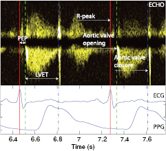
Figure 9. Annotation of aortic valve timings using Doppler mode ECHO.
Download figure:
Standard image High-resolution imageThe measurement protocol was supervised and conducted by an authorized medical specialist. It consisted of several acquisitions of ECHO in Doppler mode and PPG collected at the right-hand index finger using an infrared transmission finger probe.
A clinical expert annotated the ECHO-doppler images. The time instant corresponding to the opening of the aortic valve was defined as onset of the left ventricular outflow lobe, while the closure of the aortic valve was defined immediately before the closing click onset, produced by the residual reflux after the closure of the aortic valve cusps. An example is shown in figure 9.
In this study a total of 2081 heartbeats have been annotated, of which 1109 beats correspond to healthy volunteers and 972 beats correspond to CVD subjects.
3.1.2. Protocol for the assessment of blood pressure and vascular tone surrogates.
The data screened in this paper for the assessment of blood pressure and vascular tone surrogates was acquired in a study at the Heinrich-Heine University Hospital Düsseldorf, Division of Cardiology, Pneumology and Angiology aiming at the collection of bio-signals for the development of algorithms capable of detecting and predicting hemodynamic instability in patients suspected to be at risk for a sudden loss of consciousness.
In this study, 55 patients with unexplained syncope were scheduled for diagnostic head-up tilt table tests (HUTT), following the recommendations of the European Society of Cardiology (ESC). The study was approved by the local ethics committee and complied with international standards (ClinicalTrials.gov identifier: NCT01262508). All volunteers gave written informed consent to participate.
The HUTT protocol consisted of four phases: (1) the patient was at rest in supine position for at least 15 min; (2) the patient did a passive standing exercise (70°) for 20 min; (3) in the absence of syncope, phase (2) was extended by 15 min with sublingual administration of min 400 μg of glycerol trinitrate (GTN); (4) the patient was tilted back to a supine position. At any time, if a syncope episode occurred, the patient was brought back to a supine position immediately for recovery and the HUTT protocol was stopped. The nurse accompanying the study documented any prodromal symptoms (e.g. dizziness, sweat, tremor, etc) during the procedure.
Data of 12 patients had to be removed due to the presence of heart rhythm other than sinus rhythm or poor data quality in BP and PPG signals. The characteristics of the resulting study population consisting of 43 patients are summarized in table 3.
Table 3. Characteristics of the volunteers enrolled in the study for the assessment of blood pressure and vascular tone surrogates.
| Tilt positive (#21) | Tilt negative (#22) | |
|---|---|---|
| Age [y] | 57 ± 18 | 63 ± 17 |
| Weight [kg] | 86 ± 15 | 74 ± 13 |
| BMI [kg m−2] | 27.1 ± 4.6 | 26 ± 5 |
| Male/female | 13/8 | 10/12 |
| GTN |
15/6 | 15/7 |
The ECG and PPG signals were acquired by using a Philips MP50 patient monitor and stored on a laptop. Blood pressure was continuously measured (beat-to-beat) using a 'Taskforce Monitor' (Millasseau et al 2002). Data coming from both systems were aligned in time via the synchronously detected ECG signals. Details of the acquisition system can be found in (Couceiro et al 2013).
3.2. Data synchronization
The synchronization of the data obtained during the before mentioned studies was performed using an algorithm based on the minimization of the error between the RR intervals time series assessed from the ECGs of both systems, using the minimum least squares error criterion. Let RR1(k), k = 1,..., K, and RR RR2(m), m = 1,..., M (K < M) be the RR intervals time series of the ECGs to be synchronized. The time instant t at which both time series are synchronized is:


where  is the synchronization time series.
4. Results and discussion
4.1. Estimation of left ventricular ejection time
The algorithms' performance for LVET inference was analyzed for the whole dataset described in section 3.1.1, referred to as global dataset in the following, and in the two subsets that compose it. These are the subset of healthy volunteers, called the healthy subset, and the subset of volunteers with cardiovascular diseases, called the CVD subset.
To evaluate the performance achieved by the proposed algorithm, four performance metrics have been adopted. Let LVETMEAS:{LVETc1,..., LVETc6, LVETCHAN} be the measured beat-to-beat LVET values, corresponding to estimate 1–6 and the LVET obtained using the algorithm proposed by Chan et al (2007), respectively, and LVETECHO be the reference beat-to-beat LVET values assessed using ECHO-doppler. The abbreviation 'Error' stands for the error between measured and reference values ( ), while 'Abs. Error' concerns to the absolute estimation error (
 ). The 'Abs. Error Perc.' stands for the percentage of absolute estimation error (
 ). The agreement between measured LVET and LVETECHO was analyzed by assessing the correlation coefficients between the two variables in each dataset (Global, healthy and CVD). Additionally, the correlation coefficients were also calculated for each volunteer and the average and standard deviation over each dataset was calculated. The Pearson correlation coefficient was calculated if the variables were normally distributed, while Spearman's correlation coefficients were used otherwise. The p-values corresponding to the coefficients shown in table 4 were low (p < 0.05), enabling the rejection of the hypothesis of no correlation.
Table 4. Summary of the results achieved by the proposed LVET estimation algorithm and the algorithm proposed by Chan et al (2007).
| Context | Measured LVET | Error (msec.) Avg ± std | Abs. Error (msec.) Avg ± std | Abs. Error (%) Avg ± std | ρ | ρ Avg ± std | Range |
|---|---|---|---|---|---|---|---|
| Global | LVETCHAN | 18.75 ± 19.78 | 23.01 ± 14.60 | 8.19 ± 5.20 | 0.75 |
0.58 ± 0.19 | [186.2;388.9] |
| LVETc1 | 22.35 ± 23.91 | 28.43 ± 16.21 | 10.19 ± 5.81 | 0.70 |
0.56 ± 0.16 | ||
| LVETc2 | 22.66 ± 19.68 | 26.13 ± 14.76 | 9.37 ± 5.29 | 0.77 |
0.56 ± 0.17 | ||
| LVETc3 | 47.02 ± 23.93 | 47.74 ± 22.46 | 17.12 ± 8.05 | 0.75 | 0.55 ± 0.16 | ||
| LVETc4 | − 6.57 ± 24.09 | 18.72 ± 16.51 | 6.71 ± 5.92 | 0.70 |
0.59 ± 0.18 | ||
| LVETc5 | 75.9 ± 23.99 | 75.96 ± 23.78 | 27.24 ± 8.53 | 0.68 |
0.54 ± 0.15 | ||
| LVETc6 | − 6.22 ± 19.63 | 15.41 ± 13.66 | 5.53 ± 4.9 | 0.78 |
0.58 ± 0.17 | ||
| Healthy | LVETCHAN | 31.19 ± 12.26 | 31.03 ± 12.66 | 11.7 ± 4.61 | 0.71 |
0.48 ± 0.11 | [186.2;318.6] |
| LVETc1 | 36.15 ± 14.84 | 36.7 ± 13.43 | 13.85 ± 5.07 | 0.84 | 0.45 ± 0.1 | ||
| LVETc2 | 31.69 ± 13.92 | 31.99 ± 13.21 | 12.07 ± 4.99 | 0.86 | 0.5 ± 0.14 | ||
| LVETc3 | 57.09 ± 18.51 | 57.12 ± 18.43 | 21.56 ± 6.96 | 0.76 | 0.52 ± 0.14 | ||
| LVETc4 | 7.63 ± 14.38 | 12.91 ± 9.91 | 4.87 ± 3.74 | 0.73 |
0.49 ± 0.14 | ||
| LVETc5 | 85.76 ± 18.91 | 85.76 ± 18.91 | 32.37 ± 7.14 | 0.74 | 0.48 ± 0.11 | ||
| LVETc6 | 3.03 ± 13.66 | 10.88 ± 8.79 | 4.11 ± 3.32 | 0.72 |
0.52 ± 0.15 | ||
| CVD | LVETCHAN | 6.49 ± 15.93 | 13.48 ± 10.68 | 4.52 ± 3.58 | 0.88 |
0.66 ± 0.2 | [213.5;388.9] |
| LVETc1 | 7.19 ± 20.16 | 17.75 ± 11.95 | 5.99 ± 4.04 | 0.84 |
0.67 ± 0.14 | ||
| LVETc2 | 11.59 ± 19.39 | 18.72 ± 12.63 | 6.32 ± 4.27 | 0.84 |
0.61 ± 0.19 | ||
| LVETc3 | 34.69 ± 23.38 | 36.07 ± 21.2 | 12.18 ± 7.16 | 0.81 |
0.59 ± 0.18 | ||
| LVETc4 | − 21.94 ± 20.16 | 23.99 ± 17.67 | 8.1 ± 5.97 | 0.84 |
0.69 ± 0.15 | ||
| LVETc5 | 63.82 ± 23.37 | 63.9 ± 23.16 | 21.58 ± 7.82 | 0.80 |
0.61 ± 0.17 | ||
| LVETc6 | − 17.65 ± 19.04 | 20.63 ± 15.75 | 6.97 ± 5.32 | 0.85 |
0.63 ± 0.18 |
aEstimated values using Spearman's correlation. Note: all the presented values are statistically significant.
The agreement between  and
and  was also analyzed using regression plots (figure 10) and a Bland–Altman plot (figure 11). Error distributions were tested for Gaussianity by using the Kolmogorov–Smirnov test. Accordingly, statistical analysis was performed using the paired Student test and the two-sided Wilcoxon signed rank test and the values shown in table 4 have been found to be statistically relevant (p < 0.001).

Figure 10. Regression plots of LVETc6. (a) Healthy subset (ρ = 0.72): best linear fit y = 12.05 + 0.94x. (b) CVD subset (ρ = 0.85): best linear fit y = 34.27 + 0.94x.
Download figure:
Standard image High-resolution image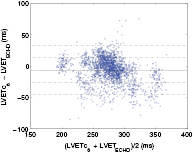
Figure 11. The Bland–Altman plot of the measured (LVETc6) and reference LVET using the proposed algorithm in the global dataset.
Download figure:
Standard image High-resolution imageIn table 4 we present the results achieved by our algorithm approach for all extracted LVET estimates. One observes that the best estimation performance was achieved by the LVETc6 estimate (measured between D2sp and D1nt), with an absolute estimation error of 15.41 ± 13.66 ms. This error translates to a percentage of error of 5.53 ± 4.9% which is comparable to the inter-observer variability (3.6%–5.4%) of Doppler echocardiographic LVET measures reported in literature (Sohn and Kim 2001, Tekten et al 2003, Colan et al 2012). The performance of the remaining estimates in the global dataset, are much less good ranging from 26.13 ± 14.76 to 75.96 ± 23.78 ms. An exception is observed for the LVETc4 estimate (measure between D2sp and D3dp) that obtained an absolute estimation error of 18.72 ± 16.51 ms, representing an increase in the estimation error percentage of about 1% (3 ms). The correlation between the measured LVET estimates and the echocardiographic LVET reference was high and ranged from 0.68 (LVETc5) to 0.78 (LVETc6).
The results regarding the evaluation of the proposed LVET estimates in both healthy and CVD subsets are also presented in table 4. In the healthy subset, we observed a decrease in the absolute estimation performance of about 5 ms for both LVETc4 and LVETc6, representing a reduction of about 1–2%. Contrarily, a decrease in the performance of the remaining estimates was observed for this subset, with an increase in the estimation error ranging from 3 to 5%. The agreement between both measure and reference LVET's increased for all the LVET estimates, with an exception to LVETc6, where a decrease of about 6% was observed. Contrarily to the results observed in the healthy subset, in the CVD subset we observed a decrease in the performance achieved by LVETc4 (23.99 ± 17.67 ms) and LVETc6 (20.63 ± 15.75 ms) and a decrease in the absolute estimation error of remaining LVET estimates. Moreover, an increase in the agreement between measured and reference LVET values was also observed in this study group, being LVETc6 the estimate with highest correlation coefficient (ρ = 0.85).
The correlation coefficients calculated in a patient-by-patient basis presented results similar (but lower,≈0.15 less) to those calculated in each dataset, showing a lower agreement between the measured LVET values and the LVETECHO, which is mainly explained by the absence of marked trend within each volunteer measured values.
Comparing the best LVET estimate (LVETc6) with the LVET obtained using the algorithm proposed by Chan et al (2007), one observes that the best estimation performance was achieved by our method, which obtained better estimation performance (15.41 ± 13.66 ms versus 23.01 ± 14.60 ms) and higher correlation (0.78 versus 0.75). In the healthy context, a significant improvement as been achieved by LVETc6 (Abs. Error: 10.88 ± 8.79 ms and ρ = 0.72) compared to the algorithm by Chan et al (2007) (Abs. Error: 31.03 ± 12.66 m and ρ = 0.71). In contrast, Chan's method performs better for CVD patients compared to our implementation (13.48 ± 10.68 ms versus 20.63 ± 15.75 ms). Finally, Chan's algorithm achieved a better correlation coefficient for CVD patients (ρ = 0.88 versus ρ = 0.85). Although our algorithm achieves higher estimation error and lower correlation in the CVD dataset, the results achieved in a balanced population (global dataset) with the similar number of beats from healthy and CVD subjects suggests that our algorithm is able to perform better across large populations.
In figure 10 we present the regression plots corresponding to the best LVET estimate (LVETc6) in both healthy and CVD subsets. For the healthy subset (figure 10(a)), the best linear fit corresponds to a 0.94 slope, which is very close to unity. This agrees with the low estimation error achieved by LVETc6 and the high correlation value presented in table 4. For the CVD subset figure 10(b)), a similar slope of 0.94 was achieved, but with a greater dispersion of the reference/measure LVET pairs.
The agreement between the LVETc6 and LVETECHO was also assessed via Bland–Altman plot, presented in figure 11 for the global dataset. The horizontal solid line represents the mean error while the dashed lines denote the level of agreement between LVETc6 and LVETECHO, i.e. mean ± standard deviation and mean ±2 standard deviation. One can observe that the average error is close to zero and the estimation error is not evenly distributed around the whole range of LVET values, particularly in the higher range where a greater dispersion is shown.
The presented results show that the characteristic points that better define the onset and end of the ventricular ejection on the PPG pulse are the systolic peak defined in the second derivative and the notch defined the first derivative. Unsurprisingly, these two points do not match exactly the onset and offset of the PPG main forward wave resultant from the ventricular ejection. This can be explained by the temporal and morphological changes experienced by the main pulse as it travels from the left ventricle to the peripheral sites. The reduction of arterial compliance (O'Rourke 1995) and the increased peripheral resistance (Allen 2007), due to the changes in the arterial wall composition and the tapering of the arteries, dampens the main pulse, and therefore a temporal shift is observed in the onset and offset of the PPG pulse. Instead, the characteristic points corresponding to the boundaries of the ejection in the PPG systolic model are determined by the characteristic points corresponding to the maximum acceleration at the systolic rise of the systolic model and by the minimum velocity during its decay. Contrarily, the remaining LVET estimates calculated form the characteristic points closer to the onset/offset of the systolic model present a higher error, resulting from an overestimation.
Our results also indicate a discrepancy in the estimation of LVET within healthy and CVD patients. In the healthy dataset, the absolute estimation error achieved by LVETc6 was very low (ap. 10.9 ms), while in the CVD the absolute error almost doubled (ap. 20.6 ms) accentuated by the underestimation of the LVET (error: −17.65 ± 19.04 ms). One possible reason for the underestimation of LVET in the CVD population is the dependence of the pulse transmission on the PWV. One common characteristic observed in aging and in populations with cardiovascular diseases, is the increase of the pulse wave velocity, mainly due to the increase of the vascular resistance and stiffness, which leads to a faster transmission of reflected waves along the arterial pathway and early appearance in the PPG pulse (O'Rourke et al 2001, Allen 2007). With the aging of the arteries (and the presence of atherosclerosis), there is a progressively return of the reflected waves, which can arrive so early during systole that it becomes difficult to distinguish the two phases (Millasseau et al 2002). This phenomenon is believed to negatively affect the proposed algorithm in two aspects. The first is the increase in the uncertainty in the identification of the systolic and diastolic phase boundaries, which consequently affects the remaining modeling process. The second is the overestimation of the Gaussian parameters related with the reflected waves in the diastolic phase, due to the attempt of the model to fit the increased (in amplitude and length) falling edge of the diastolic phase. As a consequence of this overestimation, the amplitude and length systolic model is diminished leading to an underestimation of the LVETc6. Another characteristic that is believed to accentuate the problematic is the elongation of the systolic rising edge, commonly associated with aging. As a result of this elongation, the characteristic points corresponding to the maximum acceleration of the systolic model appear at a later instant and therefore a decrease in the LVET estimate is observed.
4.2. Assessment of blood pressure and vascular tone surrogates
In this section, we analyze the relationship between the extracted blood pressure and vascular tone surrogates with the reference blood pressure and total peripheral resistance values. The relationship was evaluated in the dataset composed by all volunteers (global dataset) and in the subset composed by volunteers where greater blood pressure changes are observed, i.e. the tilt positive group (tilt positive dataset). The relationship between variables was evaluated for the upright position phase of the HUTT protocol. The extracted reference values used in the present analysis are: systolic (SBP), diastolic (DBP) and mean blood pressure (MBP), pulse pressure (PP) and total peripheral resistance index (TPRI). These parameters were compared with the extracted surrogates, i.e. SI, T1_d, T1_2, RI, R1_d and R1_2, in order to identify the parameters that better characterize blood pressure and vascular tone changes, and their level of agreement with those parameters.
Let m = 1,..., M with M = 43 be the volunteers, xmeas = {SI, T1_2, T1_d, RI, R1_2, R1_d} the measured parameters and xref = {SBP, DBP, MBP, PP, TPRI} the reference parameters, assessed in a beat-to-beat basis. The agreement ( ) between the measured and reference parameters for each volunteer using the Pearson correlation coefficient was defined as:

In tables 5 and 6 we present the Pearson correlation coefficients ρp achieved by each extracted features and the reference parameters, for the global and tilt positive datasets. The p-values corresponding to the coefficients shown in tables 5 and 6 were low (p < 0.05), enabling the rejection of the hypothesis of no correlation.
Table 5. Correlation between the extracted (SI, T1_d and T1_2) and reference parameters (SBP, DBP, MBP, PP, TPRI).
| Parameters | Absolute correlation coefficient (ρp) | Range | ||
|---|---|---|---|---|
| SI (global/tilt positive) | T1_d (global/tilt positive) | T1_2 (global/tilt positive) | ||
| SBP | 0.41 / 0.57 | 0.39 / 0.53 | 0.43 / 0.49 | [22.3; 247.1] mmHg |
| DBP | 0.42 / 0.54 | 0.41 / 0.51 | 0.40 / 0.41 | [1.7; 141.5] mmHg |
| MBP | 0.41 / 0.57 | 0.38 / 0.53 | 0.40 / 0.43 | [8.3; 168.5] mmHg |
| PP | 0.33 / 0.41 | 0.34 / 0.39 | 0.41 / 0.47 | [0; 147.7] mmHg |
| TPRI | 0.41 / 0.51 | 0.37 / 0.46 | 0.45 / 0.46 | [215.7; 7427.2] dyne * s * m2 cm−5 |
Table 6. Correlation between the extracted (RI, R1_d and T1_2) and reference parameters (SBP, DBP, MBP, PP, TPRI).
| Parameters | Absolute correlation coefficient (ρp) | Range | ||
|---|---|---|---|---|
| RI (global/tilt positive) | R1_d (global/tilt positive) | R1_2 (global/tilt positive) | ||
| SBP | 0.40 / 0.52 | 0.36 / 0.49 | 0.21 / 0.23 | [22.3; 247.1] mmHg |
| DBP | 0.38 / 0.46 | 0.37 / 0.43 | 0.23 / 0.25 | [1.7; 141.5] mmHg |
| MBP | 0.40 / 0.52 | 0.37 / 0.44 | 0.22 / 0.24 | [8.3; 168.5] mmHg |
| PP | 0.37 / 0.44 | 0.33 / 0.40 | 0.25 / 0.26 | [0; 147.7] mmHg |
| TPRI | 0.43 / 0.5 | 0.42 / 0.45 | 0.26 / 0.27 | [215.7; 7427.2] dyne * s * m2 cm−5 |
From tables 5 and 6, one can observe that the parameter achieving the best correlation coefficient in the global dataset is the T1_2, which presented a correlation with TPRI, SBP of 0.45 and 0.43, respectively. Additionally, the parameter SI and T1_d were also moderately correlated with the reference blood pressure measurements and with the TPRI, with values ranging from 0.37 (between T1_d and TPRI) to 0.42 (between SI and DBP). Similarly, the parameters RI and R1_d also showed a good agreement with the reference parameters (excluding PP) being the highest correlation with TPRI (ρp = 0.43 and ρp = 0.42, respectively). The parameter R1_2 showed to be weakly associated with each of the reference parameters, with ρp ranging from 0.21 to 0.26.
Regarding the results in the tilt positive group, one can observe a marked increase in the agreement between the majority of the measured and reference parameters. In this group of patients, the highest agreement was found between the SI and MBP (ρp = 0.57), SBP (ρp = 0.57) and DBP (ρp = 0.54). Not surprisingly, the parameter T1_d also presented a high agreement with MBP and SBP (ρp = 0.53). The parameter most closely associated with TPRI in the tilt positive volunteers was the SI (ρp = 0.51). The parameter T1_2 showed to be more closely associated with the SBP, PP and TPRI, with a level of agreement of 0.49, 0.47 and 0.46, respectively. From table 6, one can observe a similar (but lower) agreement between the parameters RI, R1_d and R1_2 and the reference parameters, with the highest level of agreement being found between RI and SBP (ρp = 0.52) and between RI and TPRI (ρp = 0.50). The parameter R1_2 presented low correlation (![${{\rho}_{\text{p}}}\epsilon \left[0.23;0.27\right]$](https://content.cld.iop.org/journals/0967-3334/36/9/1801/revision1/pmea515695ieqn048.gif) ) with all the reference parameters.
) with all the reference parameters.
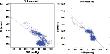
The level of agreement between the surrogates presents the best results (i.e. SI) and the SBP are illustrated by the regression plots present in figures 12(a) and (b), for two volunteers. A linear model SBP = A * SI + B was applied on the data extracted from volunteer 7 (figure 12(a)) and volunteer 36 (figure 12(b)). For volunteer 7, the best linear fit corresponds to a negative slope A = −1.8, which is very far from the unit. For volunteer 36, the best linear fit corresponds to similar slope A = −2.28. From figure 12 it is possible to observe a strong linear and negative correlation between SI and SBP, especially for lower values of SBP (high values of SI). The higher dispersion SI/SBP points for high SBPs, particularly above 130 mmHg, suggest a higher uncertainty in the SI measurement, resulting from the increasingly overlapping of the forward and reflected waves.
Figure 12. Regression plots of SI-SBP. (a) Volunteer #07 (ρ = 0.0.64): best linear fit SBPe = −1.8* SI + 491. (b) Volunteer #36 (ρ = −0.84): best linear fit SBPe = −2.28* SI + 565.6.
Download figure:
Standard image High-resolution image
The results presented in this section suggest that the extracted parameters can be associated with changes in blood pressure and vascular resistance. The presented results regarding the SI and T1_d parameters for SBP, DBP and MBP are consistent with those found by Millasseau et al (2003) (ρp = 0.48/0.68/0.51 for SBP/DBP/MDP), by Padilla et al (2009) (ρp = 0.41/0.40/0.44 for SBP/DBP/MDP) and by Brillante et al (2008) (ρp = 0.42/0.52/0.51 for SBP/DBP/MDP). Contrarily, the low agreement between RI and blood pressure measurements reported by in (Millasseau et al 2003, Brillante et al 2008, Padilla et al 2009) ( < 0.18 for SBP,
  < 0.28 for DBP and
  < 0.24 for MBP) was not found in our analysis, where the correlation found with SBP, DBP and MBP was above 0.38 for the global dataset and above 0.46 for the tilt positive dataset. The low correlation found between the R1_2 and SBP was not consistent with the association between reported by Baruch et al (2011). This discrepancy is mainly explained by the normalization of the PPG pulse performed in the present study, and by the modalities used in the study reported in (Baruch et al 2011). While Baruch et al (2011) used the absolutes amplitudes of the main forward and first reflection waves (assessed from the arterial blood pressure waveform) to estimate R1_2, in the present study the R1_2 parameter was assessed from the normalized pulse (assessed from the photoplethysmogram). The lower correlation between SI, T1_d and PP (
 ) found in the present study is in agreement with that found by Padilla et al (2009) (
 ), but not with the association outlined in (Baruch et al 2011).
The increase in the agreement between the SI, RI and the reference parameters, from the global dataset to the tilt positive dataset, show the importance of these parameters in the assessment of blood pressure and vascular tone changes, especially in cases where acute vasodilatation is present, which is the case of the patients suffering from syncope (tilt positive group).
5. Conclusions and outlook
The PPG is a promising tool to deploy solutions for ambulatory and personal health applications. Its successful utilization still lacks convincing signal processing methods that are reliable and accurate enough for the extraction and sophisticated interpretation of PPG waveform characteristics, beyond simple heart rate determination.
In the present study, an algorithm for the extraction of cardiovascular performance surrogates from the PPG waveform is introduced. The proposed methodology is based on the segmentation of the PPG signal, and consequently modeling each PPG pulse as a sum of five Gaussian functions. Using the reference echocardiographic LVET values extracted using ECHO from 68 healthy and cardiovascular-diseased volunteers, we were able to evaluate the performance of six LVET estimates. The best LVET estimate (LVETc6) achieved a low estimation error (ap. 15 ms) and a high correlation (ρ = 0.78) on a dataset composed by 2081 annotated heartbeats. Although LVETc6 did not present the best estimation error for the population with cardiovascular diseases, the high correlation (ρ = 0.85) with the reference LVET was still achieved, supporting the use of the PPG for the assessment of LVET changes. Moreover, the percentage of error in the global population below 30% suggests that the LVET can be used in the accurate determination of cardiac performance indexes (such as the cardiac contractility index and the myocardial performance) and cardiac output monitoring in p-health systems (Critchley 2011).
The relationship between the amplitude and location of the MG model waves was also investigated in the current paper, leading to the definition of six parameters related to stiffness and reflection indexes. Their relationship with reference values of blood pressure and total peripheral resistance extracted from a Taskforce Monitor was evaluated in the tilt positive group. We were able to conclude that the extracted surrogates are associated with both changes in blood pressure and total peripheral resistance. T1_2 index was found to have the highest correlation within the overall dataset, presenting a moderate agreement with the total peripheral resistance ( ) and with SBP (
 ). Moreover, a similar agreement was found between SI and the reference parameters (excepting PP), with the coefficients ranging from 0.41 to 0.42. In the tilt positive group, the stiffness index presented the highest agreement with mean blood pressure and systolic blood pressure (
 ). Although this surrogate exhibits a good level of agreement with the majority of the remaining reference parameters (
 0.51 to
  0.57), a lower correlation was found with the pulse pressure (
 0.41). Moreover, an exception was also observed for the parameter R1_2, corresponding to the amplitude ratio between the main forward pulse and the first reflection at the renal reflection site, which exhibit a low correlation with all the reference parameters (
 0.22). The results obtained during the current analysis suggest that the stiffness and the reflection indexes can be robustly estimated from the analysis of the systolic and diastolic components of the proposed model. Although the analyzed parameters do not meet standards for clinical guidance, the good correlation with the reference parameters suggest that these indexes can provide valuable information about blood pressure and vascular tone changes and especially in patients presenting hemodynamic instability. One example of a potential application of these indexes is the prediction of syncope, which is characterized by an abrupt decrease of blood pressure before its onset.
The extraction of these parameters gains a special emphasis when considering the development of p-health applications, where non-invasive, inexpensive and easy-to-use devices are essential. Unlike the state of the art continuous blood pressure monitors, the PPG is simple, low-cost and operator independent, enabling its application in a wider range of environments (e.g. home care). These advantages are highlighted by the increasingly interest in the usage of PPG in p-health devices (e.g. smart watches), which could be a potential application of the proposed algorithm. In order to analyze the PPG from such devices a special concern should be placed on the algorithms adaptation depending on the sensors light properties and acquisition site, which are known to affect the signal morphology and quality. Additionally, the selection of an appropriate temporal resolution (at least 125 Hz) should also be taken into consideration. Since the proposed algorithm is based on determination of the characteristic points from higher order derivatives, it is expectable that lower sampling rates will have a negative impact in the algorithms performance.
Acknowledgments
The authors would like to express their gratitude for the support from Centro Hospitalar de Coimbra and specially the efforts of Dr L Marques in facilitating the arrangements for the data acquisition component of the present study. We also thank S Gläser for excellent technical support.
This work was supported by CISUC (Center for Informatics and Systems of University of Coimbra) and by EU projects HeartCycle (FP7-216695), HeartSafe (PTDC-EEI-PRO-2857-2012) and iCIS (CENTRO-07-ST24-FEDER-002003).
J M is employed by Philips Research in the Netherlands.
CM and CE are funded by the Research Committee of the medical faculty of the University of Düsseldorf. CM also holds a research grant from Biotronik and the Hans-und-Gertie-Fischer-Stiftung.