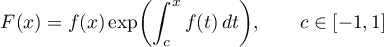
Abstract
We consider the problem of best uniform approximation of real continuous functions  by simple partial fractions of degree at most
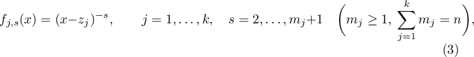
  on a closed interval
  of the real axis. We get analogues of the classical polynomial theorems of Chebyshev and de la Vallée-Poussin. We prove that a real-valued simple partial fraction
  of degree whose poles lie outside the disc with diameter , is a simple partial fraction of the best approximation to if and only if the difference
  admits a Chebyshev alternance of
  points on . Then is the unique fraction of best approximation. We show that the restriction on the poles is unimprovable. Particular cases of the theorems obtained have been stated by various authors only as conjectures.
Export citation and abstract BibTeX RIS
§ 1. Introduction. Statement of results
We study the best uniform approximation of real-valued continuous functions on closed intervals of the real axis by real-valued simple partial fractions (s. f.). Recall that a real-valued simple partial fraction of degree ,  , is the logarithmic derivative of an algebraic polynomial of degree with real coefficients:

Thus  and
and
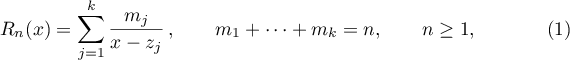
where the poles  are all pairwise- distinct zeros of the polynomial
  , and the numbers
  are their multiplicities. Clearly, the zeros are symmetric with respect to the real axis and the multiplicities of complex- conjugate zeros coincide.
Consider a simple partial fraction of order at most of the best uniform approximation of a function on a closed interval ![$S=[x_0-r,x_0+r]$](https://content.cld.iop.org/journals/1064-5632/79/3/431/revision1/IZV_79_3_431ieqn13.gif) ,
,  . We denote it by

and sometimes call this fraction optimal.
Simple partial fractions were used by Macintyre and Fuchs (1940), Gonchar (1950s) and Dolzhenko (1960s) in connection with extremal problems in classes of rational functions. As an independent tool of approximation, simple partial fractions were first used by V. I. Danchenko and D. Ya. Danchenko (1999). The theory of approximation by simple partial fractions and their modifications was further developed by V. I. Danchenko, Borodin, Kosukhin, Protasov, Kayumov, Novak and others. Some of these papers are listed in the references. For example, analogues of the classical polynomial theorems of Mergelyan, Jackson, Bernshtein, Zygmund, Dzyadyk and Walsh were obtained for s. f. (see [1], [2]). On the other hand, there are a number of principal approximative properties that do not hold for polynomials. One such property of simple partial fractions is the possibility of approximation on unbounded sets (see [3]–[6]).
Another principal feature is that the fraction  is, generally speaking, non-unique and cannot be characterized by the number of alternance points 1 for
  . The non-uniqueness of
  even in the presence of an alternance of
  points (as well as the non-necessity of such an alternance for the best approximation) was first shown in [7] by an example for
  . This example was completely generalized to
  in [8] and to arbitrary
  in [9]. Thus for s. f. there is no exact analogue of Chebyshev's classical theorem on alternance (see [10], p. 69). Our main result (Theorem 1) is an analogue of Chebyshev's theorem under an additional restriction on the poles of the simple partial fraction that delivers the alternance. Many authors have sought such an analogue, and a number of general conjectures were stated in [11]–[14]. Some of them will be established here for the first time.
The following conjecture of V. I. Danchenko [12] is still open: for every continuous function , the fraction is unique and is characterized by an alternance of  points whenever the degree
  is sufficiently large. This conjecture has been proved only for constant functions
  (see [7], [15], [16]). We note that the problem of the best approximation of constants by simple partial fractions is one of the possible analogues of Chebyshev's problem on the monic polynomial of a given degree with least deviation from zero.
We now state our results. Let be a continuous real function on the closed interval , and let  be the closed disc with diameter :

Theorem 1. If all poles of a real-valued s. f. of degree of the form (1) lie outside the disc , then  if and only if the difference
  admits an alternance of points on . In this case is the unique fraction of best uniform approximation in the class of all s. f. of degree at most . The condition on the position of the poles cannot be weakened.
The impossibility of weakening the condition on the poles means that if at least one pair of complex- conjugate poles of the fraction of best approximation lies in the disc , then, generally speaking, the best approximation is non-unique and is not characterized by an alternance of points in . Examples are given in §2.
In Theorem 1, the degree of the s. f. of best approximation is fixed (and is equal to ). In the next theorem we get rid of this restriction as far as the sufficiency of the alternance is concerned. The condition also seems to be redundant as far as the necessity of the alternance and the uniqueness of the best approximation are concerned.
Theorem 2. If a simple partial fraction  of degree
  has no poles in the disc and the difference
  has an alternance of points on , then
 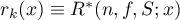 .
.
Theorem 2 is proved in §4. Theorem 1 is proved in §3 (sufficiency of the alternance) and §5 (necessity of the alternance and uniqueness of the best approximation).
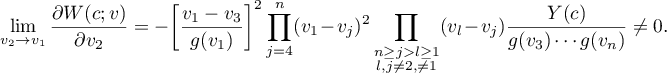
Remark 1. In the case of distinct poles of , Theorem 1 was stated and proved by the author in [14] (sufficiency of the alternance) and [17] (necessity of the alternance and uniqueness of the best approximation). We now do not require all poles to be distinct. This form of the criterion was announced by the author in [16]. Novak [11] had earlier proved an analogue of Theorem 1 in the case of distinct real poles except for the uniqueness assertion. The proofs in [11], [14], [17] make essential use of the determinant identity (8), which was conjectured (in other terminology) in [11] and verified only for small . The author has learned that (8) was proved for all by Borchardt (see [18], Russian p. 18). This promotes the previous results from conjectures to fully fledged theorems. In this paper we also use Borchardt's identity.
Remark 2. For  it is still an open question whether one can replace the disc in Theorem 1 by a smaller figure containing the closed interval . Such a replacement is impossible for because of the non-uniqueness example in [7], where the poles of each s. f. of degree 2 of the best approximation to
  ,
, ![$x\in [-1,1]$](https://content.cld.iop.org/journals/1064-5632/79/3/431/revision1/IZV_79_3_431ieqn39.gif) , lie precisely on the unit circle.
, lie precisely on the unit circle.
Remark 3. The requirement of the continuity of in Theorem 1 is redundant in the following sense. Let and  be bounded functions. We put
  and say that points
  of the closed interval form a generalized alternance on for the difference
  if every point
  is contained in an arbitrarily small subinterval
  such that at least one of the two following alternances holds:
If we define the alternance in this way, then Theorem 1 holds for all bounded functions . Only the slightest changes are needed in the proof.
As an application of Theorem 1, we consider the problem of the best approximation of continuous functions whose modulus is small on the interval ![$x\in [-1,1]$](https://content.cld.iop.org/journals/1064-5632/79/3/431/revision1/IZV_79_3_431ieqn44.gif) . We recall that Kosukhin [2] established, under very general assumptions, a connection between the least deviations from polynomials and simple partial fractions. To state his result in the case of approximation on
. We recall that Kosukhin [2] established, under very general assumptions, a connection between the least deviations from polynomials and simple partial fractions. To state his result in the case of approximation on ![$[-1,1]$](https://content.cld.iop.org/journals/1064-5632/79/3/431/revision1/IZV_79_3_431ieqn45.gif) , we put
, we put
( is fixed). Let
  (resp.
  ) be the least deviation on of from simple partial functions of degree at most (resp. of
  from algebraic polynomials of degree at most
  ) and let
  be the uniform norm on . Put
  . Then the following estimate holds (see [2]):

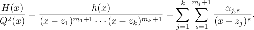
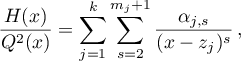
By definition we have  , where
 ![$R^*(x)\equiv R^*(n,f,[-1,1];x)$](https://content.cld.iop.org/journals/1064-5632/79/3/431/revision1/IZV_79_3_431ieqn54.gif) . Therefore,
. Therefore,

Furthermore, it is proved in [19] that the poles of every s. f. of degree satisfying the condition  for some
  lie in the exterior of the ellipse
The interior of this ellipse contains the unit disc if  . Therefore we obtain the following corollary from Theorem 1 and the previous estimates.
Corollary 1. Suppose that the following inequality holds for some constants ![$c\in[-1,1]$](https://content.cld.iop.org/journals/1064-5632/79/3/431/revision1/IZV_79_3_431ieqn58.gif) (see the definition of
(see the definition of  , and
, and  :
:

and the s. f. ![$R^*(n,f,[-1,1];x)$](https://content.cld.iop.org/journals/1064-5632/79/3/431/revision1/IZV_79_3_431ieqn61.gif) has degree . Then the best approximation is unique and the difference
has degree . Then the best approximation is unique and the difference  admits an alternance consisting of points of .
In §2 we apply this result to a concrete function (see the example in §2.4). Note that if this inequality holds, then the function itself has small modulus since we necessarily have  .
.
A lower bound for the least deviation can be obtained from the following analogue of de la Vallée-Poussin's polynomial theorem (see [10], pp. 63–64).
Theorem 3. If the poles of a s. f. of degree lie outside the disc and there are points  on the closed interval such that
  ,
,  ,
,  , then

Theorem 3 is proved in §4. Note that Theorem 3 with  was obtained in [11] (see also [14]) under some additional assumptions (see Remark 1). Here we get rid of these restrictions.
The most important auxiliary tool in the proofs of Theorems 1–3 is the following Theorem 4, which can be deduced from Borchardt's identity. Theorem 4 is of independent interest. In particular, it asserts that the functions (3) below satisfy the Haar condition on . We recall some terminology in this connection (see [10], pp. 79–88).
Continuous complex functions  satisfy the Haar condition on a compact set
  (containing more than points) if every generalized polynomial of the form
  with constants
  (not all equal to 0) has no more than distinct zeros on
  . Clearly, this condition is equivalent to the inequality
  for any distinct points
  . Haar showed that it is also equivalent to the uniqueness of the polynomial
  of least deviation for all continuous functions on . In particular, if the functions
  are real and satisfy the Haar condition on a compact set
  , then the system
  is called a Chebyshev system on . Chebyshev's alternance theorem and some other results in the theory of approximation by algebraic polynomials can be transferred verbatim to the case of Chebyshev systems.
We consider a system of functions of the form
where  are distinct points which are situated symmetrically with respect to the real axis, and with every point
  we associate a number such that
  and the numbers
  associated with complex- conjugate are equal to each other.
Theorem 4. If the numbers in the definition of the system (3) of functions lie outside the disc , then the sum of the multiplicities of the zeros on of the generalized polynomial  with arbitrary numerical coefficients
  , not all equal to
  , does not exceed .
Theorem 4 is proved in §6. We mention separately the case when the functions (3) are real-valued. In this case Theorem 4 yields the following corollary.
Corollary 2. If the numbers in the definition of the system (3) are real and lie outside the closed interval , then the functions (3) form a Chebyshev system on .
This assertion was first proved in [11] (see also [14], [17]) in the case when  , that is, for the system of functions
  with distinct real poles , under the assumption that the identity (8) holds.
Unlike the Haar condition, the property of the system (3) stated in Theorem 4 restricts the sum of the multiplicities of the zeros of . In what follows we call this property the strengthened Haar condition. Chebyshev systems possessing this property (see [20], Russian p. 58) are referred to as  -systems, while arbitrary Chebyshev systems are alternatively referred to as
  -systems.
Using Theorem 4, we prove in §3 the following theorem on the uniqueness of the solution of the multiple interpolation problem. We recall that an interpolating s. f. need not be unique, in contrast to the interpolating polynomial. This was first observed for the simple interpolation problem in [21] and [11], where one can also find some uniqueness conditions in terms of the table of interpolation nodes. The issue of the unique solubility of the interpolation problem was further treated in [13], [14], [22] and elsewhere.
Theorem 5. If a real-valued s. f. of degree of the form (1) with all poles lying outside the disc interpolates a table with  pairwise- distinct nodes
  of total multiplicity , that is,

then is the unique interpolating fraction in the class of all s. f. of degree  for all possible nodes
  , values
  and multiplicities
  .
.
§ 2. Examples relating to the main theorem
In §§2.1–2.3 we establish the unimprovability of the condition on poles in Theorem 1. In §2.4 we give an example relating to Corollary 1. The example in §2.5 concerns the case when the best approximation is attained at a s. f. with one pole.
2.1.
We show by an example that if at least one pair of complex- conjugate poles of a s. f. possessing an  -point alternance lies in the disc , then the fraction need not be optimal.
Consider a s. f.  of degree
  with poles
  and
and  , and take the interval for . Clearly, the second pair of poles lies outside the closed unit disc, and the first pair lies inside.
The function has exactly five points of local extremum on :

(alternately minima and maxima) and takes the following values  at these points:

We put  and define a continuous piecewise-linear function
  by letting it be constant on the intervals
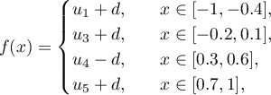
and connecting the neighbouring endpoints of these intervals by straight lines on the remaining part of .
By construction, the  points
  form an alternance for
  on and we have
 ![$\max_{x\in[-1,1]}|f(x)-R(x)|=d$](https://content.cld.iop.org/journals/1064-5632/79/3/431/revision1/IZV_79_3_431ieqn108.gif) . Nevertheless, is not a fraction of best approximation for . For example, we easily verify that the s. f.
. Nevertheless, is not a fraction of best approximation for . For example, we easily verify that the s. f.  with poles
  and
and  is a better approximation to :
 ![$\max_{x\in[-1,1]}|f(x)-\widetilde{R}(x)|=1.4427864\ldots<d$](https://content.cld.iop.org/journals/1064-5632/79/3/431/revision1/IZV_79_3_431ieqn112.gif) .
.
2.2.
The hypothesis of Theorem 1 on the position of the poles does not hold in the known examples of non-uniqueness of best approximation (see [7]–[9]). We recall that for every (see [7], [8] for small and [9] for arbitrary ) one can find an interval  , a continuous function
  and a family (with parameter
  ) of simple partial fractions
  of degree such that every fraction provides the best approximation of
  in the class of all s. f. of degree at most on . Moreover, there is a value
  of the parameter such that
  has exactly alternance points on . For all other values of the parameter, the alternance contains fewer than points.
Thus, if the condition on the position of the poles does not hold, then
(a) neither -point alternance nor uniqueness can be guaranteed for the optimal fraction;
(b) an -point alternance does not guarantee uniqueness.
The conclusions (a), (b) hold even in the case when only one pair of complex- conjugate poles of the fraction lies in the disc  (for example, this is obvious when ).
2.3.
Following [13], [8], we construct for every  an example showing that if all poles of the fraction lie in the disc , then even the presence of an alternance of
  points does not guarantee that the approximation is optimal.
It is proved in [13] that for all  and there are real polynomials and
  of degree which are positive on and such that the polynomial
  has exactly
  simple zeros on the interval
  .
.
Indeed, suppose for example that  is even, choose points
  on the interval and put

The polynomial  has at least distinct zeros on the closed interval
 ![$[x_1,x_m]$](https://content.cld.iop.org/journals/1064-5632/79/3/431/revision1/IZV_79_3_431ieqn131.gif) . These are the
. These are the  zeros
zeros  and at least one zero on each of the
  intervals
  (since the signs of the derivatives
  coincide). We similarly see that has at least distinct zeros on
 ![$[y_1,y_m]$](https://content.cld.iop.org/journals/1064-5632/79/3/431/revision1/IZV_79_3_431ieqn137.gif) . Since the polynomial is of degree , it has no zeros other than those listed, and all the listed zeros are simple. Putting
. Since the polynomial is of degree , it has no zeros other than those listed, and all the listed zeros are simple. Putting  and
and  , where
  is arbitrarily small, we see that the polynomials and are positive and, by continuity, the polynomials and have the same number of zeros on , that is, zeros. (A similar, but more involved, argument works for odd .)
Since  is small, it follows by continuity that all zeros of and lie inside the disc .
We now repeat an argument in [8]. Let ,  , be the zeros of
  enumerated in ascending order. Putting also
  and
and  , we have
  .
.
By construction, all the poles of the simple partial fractions  and
and  lie inside the disc but outside the closed interval , and the difference
  has exactly simple zeros on and preserves sign on each of the intervals
  ,
,  . This sign alternates from one interval to another.
There is no loss of generality in assuming that  for
for  ,
,  . We fix an arbitrary number
  and define a continuous real-valued function by the following (easily achievable) conditions:
1)  ,
,  ;
;
2)  for , ;
3)  , .
, .
Clearly, the deviation of the s. f. from on is equal to  and the difference has an alternance on consisting of the points
  . However, is not optimal because, by construction, the deviation of the s. f.
  from is strictly less than .
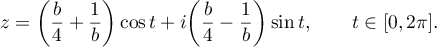
2.4.
Consider the family of functions

(where  and are parameters). The condition
  guarantees that these functions are continuous for all
  (
( ) and monotone increasing (
![$f\,'(x)= a^2e^{ax}(1- e^{ap})\times [1+ e^{ax}-e^{ap}]^{-2}\ge 0$](https://content.cld.iop.org/journals/1064-5632/79/3/431/revision1/IZV_79_3_431ieqn167.gif) ). For example, the family (5) contains all constants:
). For example, the family (5) contains all constants:  for
for  . If
. If  , then and have the same sign. Therefore, by monotonicity,
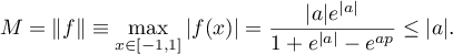
We fix a parameter ![$p\in[-1,1]$](https://content.cld.iop.org/journals/1064-5632/79/3/431/revision1/IZV_79_3_431ieqn171.gif) and put
and put  in the definition of
  (see §1). Then it can easily be seen that
  . We use the following estimate for (see [23], Russian pp. 229–230). If
 everywhere on , then

Since in our case  , we obtain
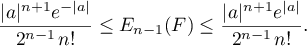
Using this and (2), we find a bound for the least deviation from  :
:

This estimate has exact order in . In particular, we obtain an estimate of exact order for the least deviations in the problem of the best approximation of constants.
Thus we have the following assertion whose last part follows from Corollary 1, the inequality  and the upper bound in (6).
Proposition 1. For all and  with , the least deviation of a s. f. of degree at most from a function of the form (5) satisfies the estimate (6), and this estimate is of exact order. If the s. f. of the best approximation of has degree for
  , then the best approximation is unique and the difference has an alternance of points on .
2.5.
Suppose that  is an algebraic polynomial of degree at most and the poles of a real-valued s. f. of the form (1) lie outside the disc . By Theorem 1 and Chebyshev's alternance theorem, the equality
  holds if and only if
  has the least deviation from on among all polynomials of degree at most . Then
  coincides with
  (the least deviation of s. f. of degree at most from ) and
  (the least deviation of polynomials of degree at most from ); compare with [13].
Theorem 2 enables us to strengthen this assertion. Namely, suppose that the poles of a s. f. of degree lie outside the disc . If is a polynomial of least deviation from on , then is a s. f. of degree of least deviation from on , and the magnitude of this deviation is  .
.
We now calculate the deviation in the case of the interval and a unipolar s. f.  ,
,  . For real and
  we have
 ![$E_{n-1}(A/(x- a),[-1,1])=|A|(a-\sqrt{a^2-1})^{n-1}/(a^2-1)$](https://content.cld.iop.org/journals/1064-5632/79/3/431/revision1/IZV_79_3_431ieqn192.gif) (this follows from [10], pp. 70–72, where this quantity is found for
(this follows from [10], pp. 70–72, where this quantity is found for  ). Using this and what was said above, we obtain the following result for the polynomial of least deviation from the fraction
  of degree :

§ 3. Sufficiency of the alternance
In this section we use Theorem 4 to prove the sufficiency of the alternance in Theorem 1. We also prove Theorem 5.
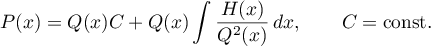
Theorem 4 is applied to simple partial fractions by means of the following lemma, which was obtained by the author [13] in the case of distinct points . We state the lemma for all simple partial fractions, although it will be used only for real-valued ones.
Lemma 1. Suppose that  , where is a polynomial of degree of the form

are distinct points and are positive integers. Then for every s. f.  of degree at most there are uniquely determined numbers such that
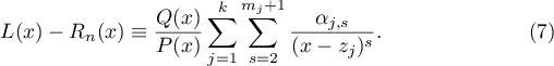
Proof. We have 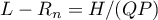 , where . Regard the formula
 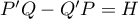 as a differential equation for an unknown polynomial of degree
  with known polynomials (of degree ) and (of degree
  ). Integrating this equation, we obtain
Clearly, each zero of of multiplicity  is also a zero of of multiplicity at least
  . Therefore
  for some polynomial
  , and the (unique) partial fraction expansion of the regular fraction
  is given by
Note that the coefficients  of the fractions
  must necessarily be equal to zero (otherwise integration gives an uncancellable logarithm, contrary to the requirement that ` is a polynomial'). Thus we have the identity
which proves the lemma. 
Here are some corollaries of Theorem 4. In their statements we assume that the s. f. are real-valued. Hence the points in the definition of  (see Lemma 1) must be situated symmetrically with respect to the real axis, and the positive integers must be equal for conjugate .
Corollary 3. If all poles of a s. f. of degree of the form (1) lie outside the disc , and if  is another real-valued s. f. of degree at most , then the sum of the multiplicities of the zeros of
  on does not exceed . In particular, the difference has at most distinct zeros on .
Proof. We have  for
for  . Hence it follows from Lemma 1 that each zero of multiplicity of is also a zero of multiplicity of the sum on the right-hand side of (7). But this sum is a polynomial in the system of functions (3) and, by Theorem 4, cannot have more than roots on (counting multiplicities).
Theorem 5 is merely a restatement of Corollary 3.
Corollary 4. If all poles of a s. f. of degree of the form (1) lie outside the disc , then the sum of the multiplicities of the zeros of the first derivative of on does not exceed . In particular,  has no more than distinct zeros on .
Proof. It follows from Corollary 3 that the polynomial has at most zeros on (counting multiplicities) if is a real polynomial of degree all of whose roots lie outside and is another real polynomial of degree at most . Putting  in the definition of , we conclude that the polynomial
 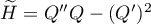 has at most roots on (counting multiplicities). It remains to note that
 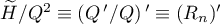 .
.
Corollary 5. (sufficiency of the alternance) Suppose that is a continuous function on the closed interval , the poles of a s. f. of degree of the form (1) lie outside the disc , and the difference has an alternance of points on . Then .
Proof. Suppose that admits an alternance of  points on the interval
 ![$S\,{=}\,[x_0-r,x_0+r]$](https://content.cld.iop.org/journals/1064-5632/79/3/431/revision1/IZV_79_3_431ieqn219.gif) . Assume that there is a s. f. of degree providing a better approximation to on than :
. Assume that there is a s. f. of degree providing a better approximation to on than :  . At the points of alternance we have
In particular, the function is continuous on and changes sign on each of the closed intervals ![$[t_j,t_{j+1}]$](https://content.cld.iop.org/journals/1064-5632/79/3/431/revision1/IZV_79_3_431ieqn221.gif) . Hence it has at least distinct zeros on the interval . By Corollary 3 it follows that
. Hence it has at least distinct zeros on the interval . By Corollary 3 it follows that  . This contradicts the assumption that is a better approximation to .
§ 4. The case of approximation by fractions of degree less than 
In this section we prove Theorems 2, 3. Since a straightforward application of the method used in §3 becomes cumbersome when the order of the approximating s. f. is less than , we prove Theorems 2, 3 in another way.
Proof. of Theorem 2 When the theorem coincides with Corollary 5 (see §3). Let us prove that an alternance of points guarantees the best approximation of by even for  .
.
Assume the opposite: there is a s. f. of degree at most which provides a better approximation, that is,  , where (here and in what follows, is the uniform norm for the closed interval ). We introduce the notation

where  ,
,  . For every such , the simple partial fraction is a best approximation to . This follows from Corollary 5 since the degree of is equal to , all its poles lie outside , and the difference
  has an alternance of points on because of the identity
  and the presence of such an alternance for
  .
.
By the triangle inequality we have the following chain:

Clearly,  and
and  decrease to zero as
  . Hence there is a
  such that
  for all
  . Thus for every we have
contrary to the assumption that is a best approximation of . Therefore our assumption is false and is indeed a best approximation to .
Proof. of Theorem 3 When the theorem is proved by contradiction in the same way as Corollary 5. We claim that the case can easily be reduced to the case as in the proof of Theorem 2. Indeed, given and , we construct a fraction and a function as above. It follows from the hypothesis of Theorem 3 and the identity that we have  , , , at the points of the interval . Since all the poles of the s. f. of degree lie outside the disc and, since the theorem is already known for fractions of degree , the following bound holds for all (see the proof of Theorem 2):

Here and in what follows we write  for the least deviation of simple partial fractions of degree at most from the function
  on .
on .
Let  be a s. f. of degree of best uniform approximation to on . Assume that
  , where . Let
  be a positive number such that
  for all
  . Then, by our assumption,

for . This contradicts the inequality  . Hence
  .
.
§ 5. Necessity of the alternance. Uniqueness of the best approximation
Here we prove the remaining assertions in Theorem 1. To simplify the notation, we assume that ![$S=[-1,1]$](https://content.cld.iop.org/journals/1064-5632/79/3/431/revision1/IZV_79_3_431ieqn246.gif) (the case of an arbitrary closed real interval is reduced to this by the linear transformation
(the case of an arbitrary closed real interval is reduced to this by the linear transformation  ).
).
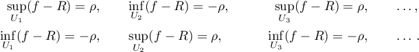
Necessity of the alternance of points. Suppose that the poles of the s. f. of degree of the best approximation to a continuous function on lie outside the disc ![$B([-1,1])$](https://content.cld.iop.org/journals/1064-5632/79/3/431/revision1/IZV_79_3_431ieqn248.gif) , and let
, and let ![$d=\max_{x\in[-1,1]}|f(x)-R_n(x)|$](https://content.cld.iop.org/journals/1064-5632/79/3/431/revision1/IZV_79_3_431ieqn249.gif) be the least deviation.
be the least deviation.
Assume that has an alternance of only  points on . Then there are points
  such that
1)  for all
  ;
;
2) for every  the difference attains an extremal value
  on the closed interval
 ![$[x_j,x_{j+1}]$](https://content.cld.iop.org/journals/1064-5632/79/3/431/revision1/IZV_79_3_431ieqn256.gif) .
.
We note that the extremum on ,  , is necessarily attained at an interior point while the extremum on
 ![$[x_1,x_2]$](https://content.cld.iop.org/journals/1064-5632/79/3/431/revision1/IZV_79_3_431ieqn258.gif) (resp.
(resp. ![$[x_m,x_{m+1}]$](https://content.cld.iop.org/journals/1064-5632/79/3/431/revision1/IZV_79_3_431ieqn259.gif) ) may also be attained at the endpoint
) may also be attained at the endpoint  (resp.
  ).
).
We first consider the case when  . Define the following -tuple of points
  :
:

where is small so that the poles of the s. f. lie outside the disc  with diameter
 ![$\widetilde{S}=[-1-\varepsilon,1+\varepsilon]$](https://content.cld.iop.org/journals/1064-5632/79/3/431/revision1/IZV_79_3_431ieqn265.gif) . For all
. For all  of sufficiently small modulus, the problem of interpolating the -node table

by simple partial fractions of degree has a unique solution  . The degree of is equal to , and the poles of lie outside the disc . This follows by continuity from Theorem 5 (see §1) since the only solution of the interpolation problem for
  is the s. f.
  .
.
Furthermore, by Theorem 5, the graphs of and for small  have no intersections on
  except for the nodes
  , and all of them are simple zeros of the difference
  . Hence the function
  , whose modulus can be made arbitrary small on by an appropriate choice of
  , preserves its sign on each of the intervals
  ,
,  ,
,  ,
, ![$(c_n,1+\varepsilon]$](https://content.cld.iop.org/journals/1064-5632/79/3/431/revision1/IZV_79_3_431ieqn279.gif) , and this sign alternates as we pass from any interval to the next. We can choose the sign of so that
, and this sign alternates as we pass from any interval to the next. We can choose the sign of so that ![$\max_{x\in[-1,1]}|f(x)-L(x;\tau)|<d$](https://content.cld.iop.org/journals/1064-5632/79/3/431/revision1/IZV_79_3_431ieqn280.gif) . This contradicts the optimality of and hence proves the necessity of the existence of an alternance of points.
. This contradicts the optimality of and hence proves the necessity of the existence of an alternance of points.
It remains to consider the case when  . We reduce it to the previous case by complementing the -tuple (defined as above) of the points , , with points
  in the interval
  . This proves the necessity of the alternance.
The uniqueness of the best approximation is proved in the same way as Corollary 5 (see §3) with the following difference. If the s. f. of degree with poles outside and another s. f. of degree are fractions of least deviation from on , then the existence of an alternance of points for on (which has been just proved) means that the difference  has at least zeros on (counting multiplicities). More precisely, the sum of the number of simple zeros and twice the number of multiple zeros is not smaller than (compare [13]). By Theorem 5 we have . This completes the proof of Theorem 1.
§ 6. Proof of Theorem 4
We divide the proof of Theorem 4 into three parts (cases). In the first and second parts we show that the system (3) satisfies the Haar condition on for and  respectively. In the third part we study the general case of the strengthened Haar condition. Note that the Haar condition for was verified in [14], but we reproduce this proof (that uses the identity (8)) for the sake of completeness.
It is convenient to prove the Haar condition (a particular case of Theorem 4) in terms of certain determinants. The fixed numbers will be referred to as poles (not points) in contrast with the variable points appearing in the statement of the Haar condition (see §1).
Theorem 4'. Suppose that for each of  distinct poles of the system of functions (3), which are situated symmetrically with respect to the real axis, we are given a number such that , and conjugate correspond to equal . If all the poles lie outside the disc , then the determinant

is different from zero for any distinct points .
Case 1 (the main case): . We denote the -tuples of the points and poles by

Since  for all
  , the system of functions (3) takes the form , and the Haar condition is written as the inequality

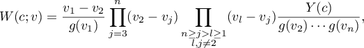
for all -tuples of distinct points on the closed interval . To prove this inequality, we use the following identity of Borchardt (1855), which was stated in the monograph [18] on permanents of matrices. (The permanent of a square matrix is the function calculated by the rule of expanding the determinant but taking the sign `plus' of every product of entries independently of the parity of the corresponding permutation.)
Borchardt's identity. For any disjoint -tuples and  of complex numbers we have

where  and are the determinant and permanent of the matrix
  respectively.
The following expansion for the determinant  is known ([10], p. 29):

where the sign  depends only on , and
  . In our case, the points and the poles are pairwise distinct, whence the factor in (8) is different from 0.
The inequality  is established in Lemma 2 below. It holds for more general -tuples and than in the inequality
  . The lemma will be proved in §7 (compare [14]). Thus we arrive at the desired inequality
  , which expresses the Haar condition for distinct poles.
Lemma 2. The permanent  of the matrix is non-zero for any -tuple of points in (not necessarily distinct) and any -tuple of poles lying outside the disc symmetrically with respect to the real axis (not necessarily distinct).
Case 2 (the general case in Theorem 4'): . We consider two basic subcases in detail.
Subcase 2.1: a real pole  is equipped with a number
  , and the poles
  are equipped with numbers . (We note that here the number of distinct poles is equal to
  since .) The functions in the system (3) take the form

The determinant in the Haar condition is correspondingly written as

We claim that  for all pairwise- distinct points
  .
.
Indeed, take pairwise- distinct points  situated symmetrically with respect to the real axis and satisfying the equalities
  ,
,  , ... ,
  . Using them and the points , we construct an auxiliary determinant
  , where
  . It is easily seen that

The identity (8) enables us to replace  in this expression by
  . We expand the derivative of this product into a sum by Leibniz' formula. Each summand is a multiple of some derivative of
  . We easily see from the definition of
  that the limiting values of all relevant derivatives of (except possibly for the highest) are equal to zero because each of these limiting values is a determinant with at least two equal columns. Hence,

But the limit of the permanent is different from zero by Lemma 2 (whose hypothesis allows for coincidence of some points inside each of the two -tuples of arguments). It remains to prove that the limit of the derivative of the determinant is non-zero. This limit can be written more conveniently as

We see from (9) that
where 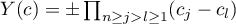 . We find the value of the innermost bracket in the limiting equality (10):
Then we calculate the limit of the second derivative of the resulting expression with respect to  and so on. Each differentiation gives rise to a non-zero quantity since one can easily see that the limit (as
  ) of the derivative of order
  with respect to
  is taken from a function of the form
  , where
 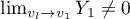 . Hence
  , as required.
Thus Theorem 4' holds under the hypotheses of Subcase 2.1.
Subcase 2.2: complex-conjugate poles and  are equipped with equal numbers
  , and the remaining poles
  are equipped with numbers . Here
  . As above, we denote the determinant in the Haar condition for the corresponding system of functions by
  and consider an auxiliary determinant with pairwise- distinct points situated symmetrically with respect to the real axis and satisfying the equalities ,
  ,
,  ,
,  , ... , . Note that the determinant coincides (up to a non-zero factor
  ) with the limit
Using (8), (9) and Lemma 2, we now see that  .
.
Thus Theorem 4' holds under the hypotheses of Subcase 2.2. In the general case 2, the theorem is proved by successive application of the scheme used in the two basic subcases to each pole with  . This completes the proof of Theorem 4'.
Case 3 (the general case of Theorem 4). Here the polynomial in the system of functions (3) may have multiple zeros. Consider the homogeneous system of equations for the coefficients obtained from (7) in view of the multiple interpolation conditions (4). It suffices to verify that the determinant  of this system is non-zero. We easily see that is equal to the limit of a certain derivative of the determinant
  (see the statement of Theorem 4') with respect to the variables . For example, if the nodes
  in the conditions (4) are simple and the node
  is double, then
  . Arguing as above, we see that
  . This proves Theorem 4 (the strengthened Haar condition).
§ 7. Proof of Lemma 2
Here we reproduce the corresponding proof from [14] almost verbatim. As in [14], we only consider the case when . Let  be the number of those real numbers that are smaller than
  (if some of the coincide, then we count each of them).
When all the numbers are real, the signs of all summands in the expansion of are equal to  and, therefore, (this was observed in [11]).
Suppose that there is at least one pair of complex- conjugate numbers . Reorder the in such a way that their list begins with all pairs of complex- conjugate numbers and ends with real numbers. Take . Under our assumptions we have  ,
,  , and the numbers
  and
and  range over . We calculate the permanent
  directly:

Since  , it follows that the inequality
  holds for all , in if and only if
We easily see that the minimum is attained at the points  and is equal to
  . Under the hypotheses of the lemma with we have
  (the points and lie outside the closed unit disc). Therefore
  . This proves the lemma for .
We now suppose that  . The determinant
  can be written by Laplace's theorem (see, for example, [24], p. 129) in the form
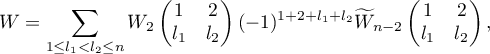
where  is the minor of order 2 formed by the entries of situated at the intersection of the first and second columns and
  th and
  th rows, and
  is the complementary minor of order
  . Thus, by the definition of the permanent, we have
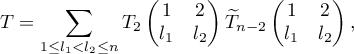
where  and
and  are the permanents of those submatrices whose determinants are equal to and respectively.
We claim that in our situation all the products  have the same sign and, therefore, the sum is non-zero. Indeed, by what was said above, we have
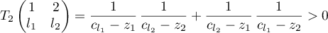
for all ![$c_{l_1},c_{l_2}\in [-1,1]$](https://content.cld.iop.org/journals/1064-5632/79/3/431/revision1/IZV_79_3_431ieqn364.gif) . Therefore the sign of the product
. Therefore the sign of the product  is equal to the sign of . If all are real except for and , then we have seen that
  . If
. If  ,
,  is the next pair of complex- conjugate poles, then the previous argument works for the permanent . After several iterations, factoring out only positive factors at every step, we exhaust all pairs of complex- conjugate . Hence only sums with real remain, and the total sign is . The lemma is proved.
Footnotes
- 1
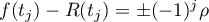
We recall that points
of form a Chebyshev alternance (in what follows, simply an alternance) on for the difference of two continuous functions and if , , where .