


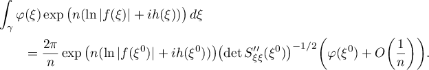
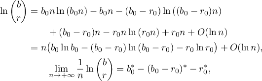
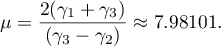
Abstract
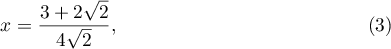
Using a new integral construction combining the idea of symmetry suggested by the second author in 2007 and the integral introduced by Marcovecchio in 2009, we obtain a new bound for the approximation of  by numbers in the field
  .
.
Export citation and abstract BibTeX RIS
| The research was partially supported by the Russian Foundation for Basic Research (project no. 12-01-00171). |
§ 1. Introduction. Integral construction. Arithmetic part
The object of this paper is to prove the following result.
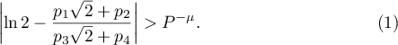
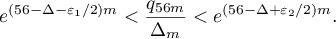
Theorem 1. Let  ,
,  ,
,  ,
,  , and
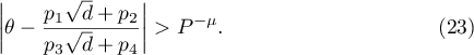
, and  . Then the following inequality holds:
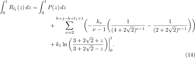
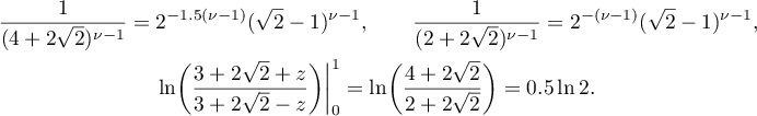
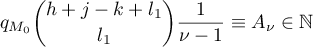
A similar bound for  was obtained in [1], and this result was improved in [2]; the corresponding value of
  was
was  .
.
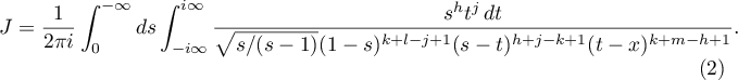
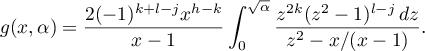
The derivation of the new bound (1) is related to an application of the following integral construction. Let  ,
,  ,
,  ,
,  and
and  . Let
. Let  ,
,  and
and  . Consider the integral
The result in Theorem 1 is obtained by taking

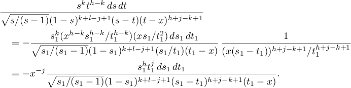
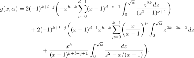
The integral (2) differs from the integral introduced by Marcovecchio in [3], p. 148, formula (5), only by the factor  in the denominator of the integrand. The integral (2) was considered for the first time in [4]. To make the picture complete, we describe a brief scheme of some transformations of this integral (see [4], Russian pp. 484, 485). We denote the integrand of (2) by
  . Then
Evaluating the residue in (5) and making the change 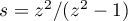 in the integral with respect to the variable
  , we obtain the relation

where

By choosing for  a value
  , we see from (5) and (6) that
We write

let  be the ring of numbers of the form
  , where
  , and for positive integers
  write
write  with
with  .
.
Lemma 1. Let  ,
,  . Then the following representation holds for all
  :
:

where the  belong to
  .
.
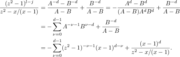
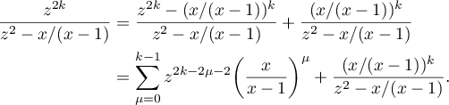
Since the integrand (8) of the integral in (10) is even, we have the following expansion into a sum of simplest fractions:
where ![$P(z)\in\mathbb{K}[z]$](https://content.cld.iop.org/journals/1064-5632/82/3/549/revision1/IZV_82_3_549ieqn39.gif) ,
,  , and, moreover,

By Leibniz' formula, we see from (12) that
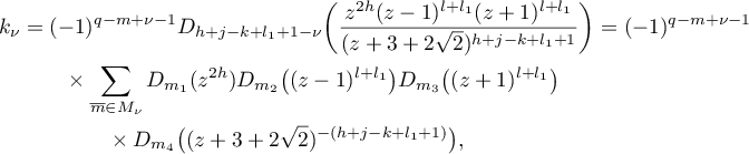
where

Therefore,
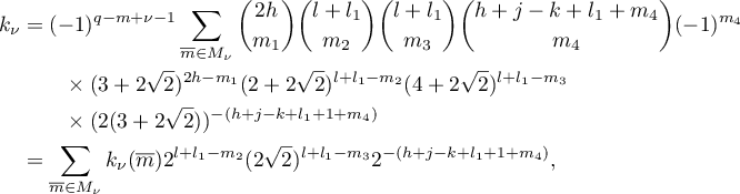
where the  belong to .
However,  . Hence,
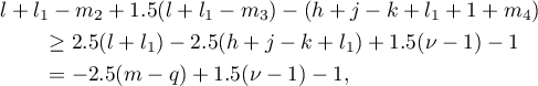
that is,

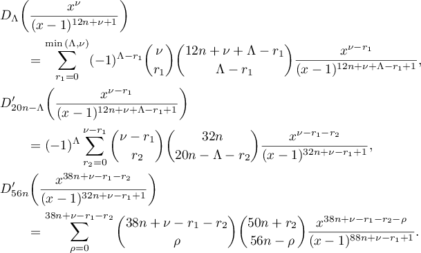
By (12), we have
Obviously,
Further, it follows from the definition of  that
that 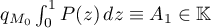 . It can also readily be seen that
for all  . Then it follows from (13) and (14) that
whence, since , (11) follows. 
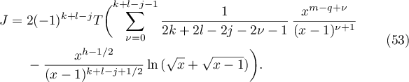
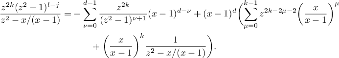
Corollary 1. The integral (2) admits the following representation for :

where  . Applying Lemma 1, we see from (7) and (9) that
where  , and this proves Corollary 1.
Along with the family of parameters (4), we shall use a more general situation in which

where  . It is convenient to denote the integral (2) for parameters of the form (16) and for
  of the form (3) as follows:

For the family of parameters (16) we write

Let  be a prime,
  , and
, and  the fractional part of the number
  . Consider the inequalities
We denote by  the product of all primes
  such that satisfies at least one of the inequalities (19). The following lemma sharpens the result obtained in Corollary 1.
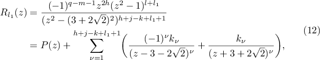
Lemma 2. When the integral (17) admits the representation

where  ,
,  .
.
Proof. The representation (20) follows from (15) by the standard procedure of refining the denominator (see, for example, Lemma 3 in [6]). The inequalities (19) were obtained for the integral (2) for the first time in [4], Russian p. 491, inequalities (11). The inequalities (19) differ somewhat from those considered, for the same purpose, by Marcovecchio in [3], inequalities (31).
The following lemma contains the final version of a linear form of the form (20) which we shall use to prove Theorem 1.
Lemma 3. The following representation holds ( see (17)):
where the  belong to
  and is defined by the inequalities (19) for the family of parameters (4).
Proof. It was proved in [4], equation (10), that the equation  holds (see (17)), that is,

For the family of parameters (4) we have from (18) that

However, then

By Lemma 2,

where , which implies (21).
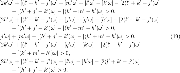
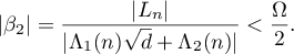
We conclude §1 by proving the following important lemma.


where the belong to , and let 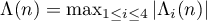 . Let
. Let

and for some constant  and every
  let there be an
  such that the following inequalities hold for every
  and at least one of the values
  :
:

Further, let  ,
,  ,
,  ,
,  ,
,  and . Then
Proof. We fix a  such that
  and write

Let us choose  ,
,  ,
,  in the inequalities (22). We introduce an
  , where
  and the following family of conditions holds: for all ,
  ,
,


Let  and . We define ,
  , by the inequalities

Then the inequalities (22) hold for at least one of the values . We write (see (25))

Let us first consider the case in which the inequalities (22) hold for  . Two situations are possible:
  ,
,  .
.
1) Let . We have
We have  by (22), and
  by (28). Hence, by (32), the condition
  and the inequality (24) yield that
which coincides with the inequality (23).
2) Let  . We consider
where

Obviously,
Therefore,

We claim that
By the inequality (33), it suffices to prove that

Applying the inequalities (22), (26), (32), (27) and (29), we obtain that

This proves the inequality (34), and therefore  . However,
  . Hence,
 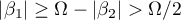 . Using the inequalities (33), (26), (27), (28) and (32) in succession and taking into account that
  , we have
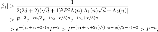
which coincides with the inequality (23).
Let us now consider the case in which the inequalities (22) hold for  . Again, two situations are possible: , .
3) Let . As in part 1), we have
Applying the inequalities (22), (28) and (30), we obtain that

4) Let . The arguments here are similar to that in part 2), where  , in particular, in the inequalities (33) and (34). Applying the inequalities (22), (26), (32) and (27), we obtain that

which proves the inequality (34) with , and simultaneously the inequality  . Then, applying the inequalities (26), (27), (28), (31) and (32) in succession, we obtain
which coincides with the inequality (23).
This completes the proof of the lemma.
Remark 1. Assertions similar to Lemma 4 were used in [1], [2] and [5].
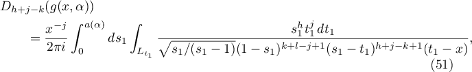
§ 2. Asymptotics
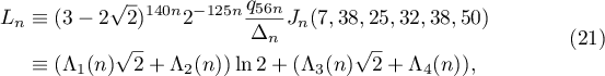
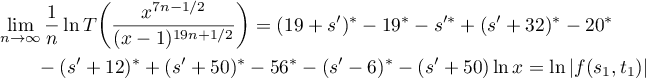
To prove Theorem 1, we shall apply Lemma 4 to the linear form (21). We need to evaluate the constants  ,
,  and
and  . In this section, we evaluate and and, in the next section, the constant . To evaluate both the constants and , we apply the saddle-point method. We have (see (17) and (21))

where
The saddle points are the solutions of the system  ,
,  that differ from the zeros of the function
  . In [4], Russian p. 492, equations (12), this system was solved in the general case for the integral (17). For the function written above we have three saddle points:


 , the complex conjugate of
  . We write
  .
.
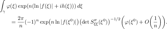
Lemma 5. Let  be a non-degenerate saddle point of the function
  , let
, let  be a two-dimensional smooth complex manifold with boundary, let be an interior point of , let the functions
  and be holomorphic at the point , and let also
  be attained only at the point , let
Then, as  ,
,

Proof. This assertion is proved in the Fedoryuk's monograph [7], p. 259, Proposition 1.1.
Lemma 6. For the linear form (21) we have the equation
Let  be the circle
  and
and  the circle
  . We note that, by (3) and (36), we have
  . Obviously,
  is attained only at the point
  . We denote by
  the image of the circle under the map
  and by
  the image of the circle under the map
  . Then it follows from the definition of the function
  that
that  is attained only at the point
  . For the integral
  , by (35), we have

where  (see Corollary 1).
We claim that
where the circles and are traversed in the positive direction. Equations of the form (41) are standard and occur in many papers, for example, in [3] and [8].
In the proof of Lemma 1, for the integral in (10) we have, by (12) and (14)
where  ,
,  and
and  , and then it follows from (7), (9) and (40) that
  . Applying (6), we obtain

where  stands for the contour going around the point
  in the positive direction and mapping onto the circle under the map . Thus, the formula (41) is proved.
Let be a small arc of the circle with centre at the point  , let be a small arc of the circle with centre at the point
  , let
, let  , let
, let  ; let
; let  , and let
  . We can define some branch
  on holomorphic at the point .
It follows from (35) and (36) that  , and therefore one can choose
  . Further, the function is holomorphic at the point since
  ,
,  . Obviously,
  . By (41) we have

We apply Lemma 5 to the first integral in (42) with  and
and  . The conditions of Lemma 5 are satisfied, since the remaining non-degeneracy condition for the saddle point can readily be verified:
  . Then by (38) we obtain
We estimate the second integral in (42) trivially:
for some positive constant  . Then
  .
.
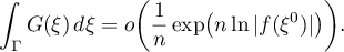
To complete the proof of the lemma, it remains to evaluate the limit
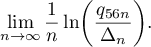
We note that  and evaluate
  . Let us write out the inequalities (19) for the family of parameters (4):
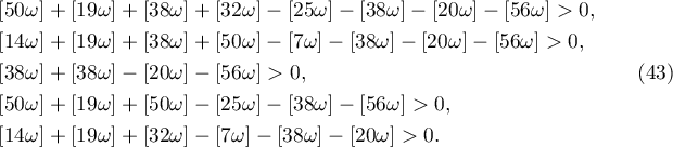
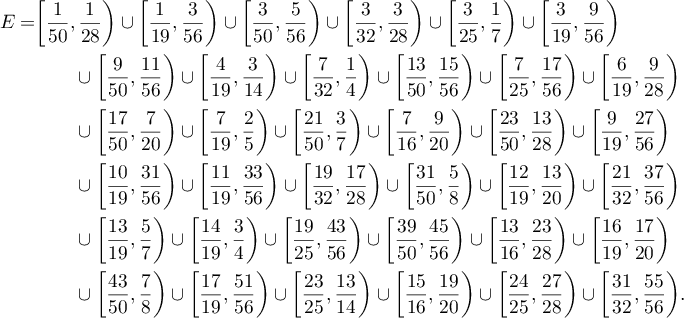
The set  of numbers
  satisfying at least one of the inequalities (43) has the form
Let  , where
  stands for the gamma function. Then, in the standard way (see Lemma 6 in [9]), we obtain
This completes the proof of the lemma.
Lemma 7. For the linear form (21) let

where the function  is defined in (35), the point
  is of the form (37), and is evaluated in (44).
Futher, let  . Then there is an
  , , such that the following inequalities hold for all and for at least one of the values :

Proof. Let  be a ray, in the complex plane , which issues from zero and passes through the point
  and let
  be an analogous ray, in the plane
  , which passes through the point
  . By (35), we have
Let  . Then
  , that is,
  . Let us move the integration with respect to in the integral
  :
:  , and let us similarly move the integration with respect to the variable :
  . Since there are no singular points of the integrand in the domains between the indicated rays, it follows that
  . Hence,
As in Lemma 6, we write  and
and  .
.
Simple computer calculations show that  is attained only at the point . Let be a small segment of containing as an interior point, let be a similar segment of containing as an interior point, and let
  ,
,  and .
and .
As in Lemma 6, one can apply Lemma 5 to the integral  , since

In our situation, the equation (38) becomes
We have 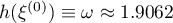 . Let
. Let 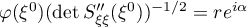 ,
,  . Then (see (47))

Obviously,
Let us write  . We claim that for every

Indeed, let  ,
,  , where
  ,
,  . If
. If  , then

In this case,  , that is,
  . Let be the value for which
  . We choose
  and
and  . Then for
  , we obtain from (17) that the integral
  has the bounds
Since  , it follows that for all
  we have
Let 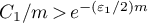 ,
,  and
and 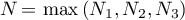 for all
  . Then, by (21), for we have

and similarly  . This completes the proof of the lemma.
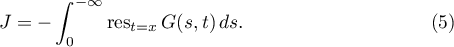
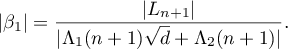
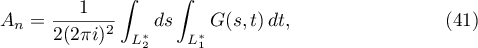
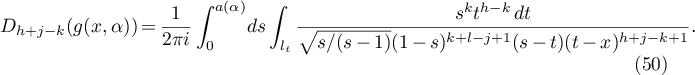
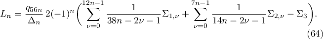
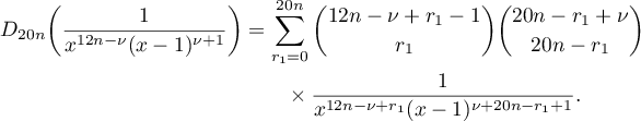
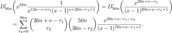
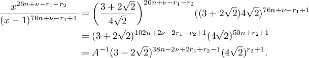
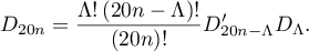
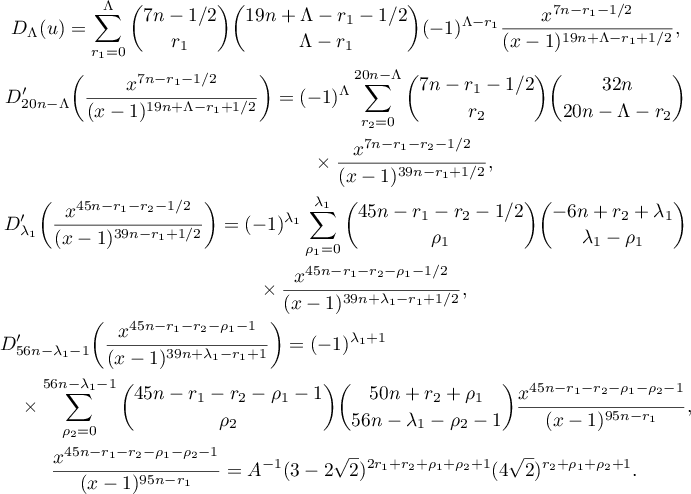
§ 3. Evaluation of the constant  . Completion of the proof of Theorem 1
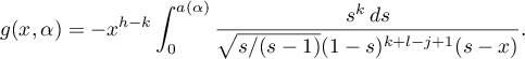
For the integral (2) we consider the function

where  ,
,  ,
,  is the circle in the complex plane whose diameter is the segment
 ![$[{x}/{2},2x]$](https://content.cld.iop.org/journals/1064-5632/82/3/549/revision1/IZV_82_3_549ieqn208.gif) on the real line, and the integration with respect to is carried out in the negative direction.
on the real line, and the integration with respect to is carried out in the negative direction.
In this section, we write

In the following lemma we establish a relationship between the function  and the integral (2).
Lemma 8. The integral (2) and the function (48) satisfy the relation

where  is the operator
  .
.
Proof. By (48), we obtain in the standard way (see, for example, [3], pp. 167–169) that
In (50) we make the change of variables  ,
,  . For all
  we obtain the integration with respect to the variable in the negative direction over the circle
  whose diameter is the segment
 ![$[2s,{s}/{2}]$](https://content.cld.iop.org/journals/1064-5632/82/3/549/revision1/IZV_82_3_549ieqn216.gif) . Further,
. Further,  ,
, 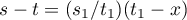 and
and 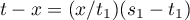 . Therefore,
The formula (50) becomes
where the integration over is carried out in the positive direction.
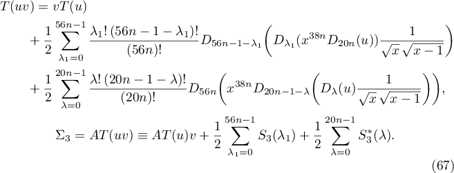
Let us multiply both the sides of the identity (51) by  and apply the operator
  to both sides. One can now replace the integration over by integration over the line
  since both integrals are equal to
 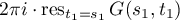 . Finally, passing to the limit as
  , we obtain the identity (49).
Our next task is to evaluate the function .
Lemma 9. The function (48) satisfies the relation

Proof. We evaluate the inner integral in (48) using Cauchy's residue theorem:
Let us make the change  in the integral thus obtained. Setting
  ,
,  ,
,  and
and ![$u\in[0, \alpha]$](https://content.cld.iop.org/journals/1064-5632/82/3/549/revision1/IZV_82_3_549ieqn229.gif) , we obtain
, we obtain
Finally, let us make the change  ,
, ![$z\in[0, \sqrt{\alpha}\,]$](https://content.cld.iop.org/journals/1064-5632/82/3/549/revision1/IZV_82_3_549ieqn231.gif) . We have
. We have
This completes the proof of the lemma.
The following lemma gives a representation of the integral (2) in a form convenient for the evaluation of the constant . We restrict ourselves to the case  , which holds for the family (4) of parameters.
Lemma 10. Let . Then the integral (2) satisfies the relation


Further,
Therefore,
Hence, it follows from (52) that
By (49), we have
We claim that 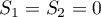 . Consider the sum
  . For all
 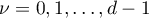 , we obtain from Leibniz' formula that
Therefore,  . Hence,
  . Similarly,
  . Further, in the sum
  we set
  ,
,  . Then
Finally,
that is,

We have  , which coincides with the assertion of the lemma.
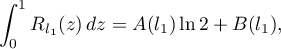
To evaluate the integral (2) by applying the formula (53), two more lemmas will be useful.


Proof. We proceed by induction on  . When
  we have
which coincides with (54) when .
Let us make the induction step  . Using the induction assumption, we obtain
We write
We need to prove that  for all
  .
.
The following equation holds:

Further,
Finally, when ![$\rho\in[1, M]$](https://content.cld.iop.org/journals/1064-5632/82/3/549/revision1/IZV_82_3_549ieqn253.gif) we need to show that
we need to show that
Consider two cases.
1. Let  . Here
Therefore,
2. Let  . Here
This completes the proof of the lemma.
Lemma 12. The following equation holds for every and for arbitrary analytic functions  and
and  :
:

Proof. By the definition of the operator  , it suffices to show that
In turn, to prove the formula (56), it suffices to prove that the coefficients of  ,
,  , on both the sides of the equation (56) coincide, that is,

We shall prove this by induction on  . When
  we have
To carry out the induction step  , note that
By the induction assumption,
and then the equation (57) holds.
In what follows, it is useful to note the asymptotics of generalized binomial coefficients:
For  we introduce the function
Obviously, the function  is odd.
Lemma 13. Let ,  ,
,  ,
,  ,
,  ,
,  and
and  . Then the following equation holds:

Proof. It is clear that  . If
. If  , then
and the formula (59) holds. Let  everywhere below. We consider several cases.
1) Let  . The following formula holds:
It follows from Stirling's formula that  as
as  . Taking into account that
  ,
,  ,
,  as , we obtain
Similar formulae hold for  and
and  . Therefore,
and the formula (59) is proved in the case under consideration.
2) Let  . Here
for some constant  , and the formula (59) is verified trivially.
3) Let  . In this case,
where, as above, the constant  is non-zero,

and we have used the fact that the function (58) is odd.
4) Let  . As in cases 2) and 3), the following equation holds:
that is,
The last case remains.
5) Let  . Here
This completes the proof of the lemma.
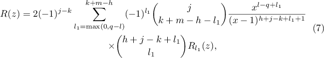
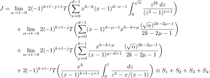
Let us apply the results thus obtained to the linear form (21). We first evaluate the integral in (35) using the formula (53):
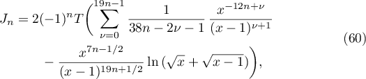
where stands for the operator  .
.
We write  and
and


Then it follows from (21) and (60)–(63) that
Let us combine the evaluation of the operators  by the ordinary Leibniz formula and by the formula (54). In the latter case, we denote the operator by
  .
.
Let us begin with the evaluation of  . We have
By Lemma 11,
Non-zero summands occur in the last sum only when ![$r_2\in[6n, 26n+\nu-r_1]$](https://content.cld.iop.org/journals/1064-5632/82/3/549/revision1/IZV_82_3_549ieqn294.gif) . Further, it follows from (3) that
. Further, it follows from (3) that
Therefore, it follows from (61) for 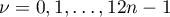 that
that
Let us now evaluate  for
for  . We write

where  ,
,  , will be chosen below to optimize the bound for .
We have
As in the evaluation of , we have

Therefore, it follows from (62) that
Finally, let us calculate the value of  using Lemma 12. We write

Then

Similarly,
We note that  .
.
Hence, the coefficient at in the linear form (21) is

Remark 2. The formula (68) enables one to find the constant (see Lemma 6) using the terms of some positive series rather than by applying the saddle-point method. The former method is very simple, and therefore it is popular. It has been used many times in recent years; see, for example, [3], [6] and [9]. Therefore, we restrict ourselves to rather brief comments.
Since  , it follows that

is a convergent series. Therefore, differentiating termwise, we obtain the positive series

The desired asymptotic behaviour is given by the maximal term of the series. Let us find this term by solving the equation
We have  . Correspondingly, the index of the maximal term of the series is
  . Therefore, as in the papers indicated above,
by Lemma 13, and, using the equation (68) we obtain the result coinciding with that of Lemma 6. We note that the reasoning used in Remark 2 does not involve the evaluation of the constant .
Let us return to the proof of Theorem 1. The first term in the sum (67) is evaluated in the same way as , where  . The half-integer value of
  enables us to extend the bounds of variation of
  ,
,  ,
,  . Instead of (66), we obtain
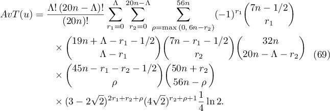
Let us now evaluate the summands  in the sum in (67). As above, let
We obtain in succession
Therefore,
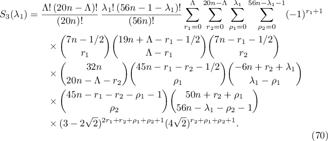
It remains to evaluate  . Let
. Let
We obtain in the standard way that
Thus, in the second case, we have
All the summands in (64) evaluated using the formulae (65), (66), (70) and (71) are of the form  or
or  , and the summands in the formula (69) are of the form
  or
or  , where
  and
and  . We note that
  and
and  for , where
  . Correspondingly,
  . Obviously,
  .
.
The total number of summands in  is estimated as
  . Thus, for we have the bound
  , where
  is the summand of maximal modulus among all above sums after replacing
  by
by  . The asymptotic behaviour of the binomial coefficients is calculated using Lemma 13.
Computer calculations show that the corresponding maximal summand is attained in the sum (69) for the following values of parameters:  ,
,  ,
,  and
and  , where

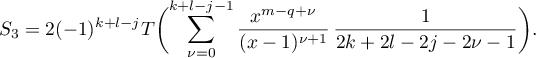
Hence by Lemma 13, it follows from (69) that
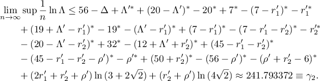
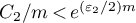
Then, by Lemma 4, the inequality (1) holds for
This completes the proof of Theorem 1.
§ 4. Concluding remarks
4.1. The number occupies a special position in the theory of Diophantine approximation. As Nesterenko said in the paper [9], `` is a natural model for comparing the different methods developed for estimating the irrationality exponent for logarithms of rational numbers''. The best estimate for the irrationality measure of the number is due to Marcovecchio [3]: 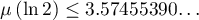 , and the estimate for the measure of quadratic irrationality is due to Polyansky [10]:
 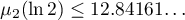 . For obvious reasons, the estimate obtained in this paper is between these values.
4.2. In [1], to obtain an estimate of the form (1), the classical hypergeometric construction with integer parameters was used, while in [2] an analogous integral (but with half-integral parameters) was applied. In essence, the integral (2) is a linear combination of hypergeometric integrals with half-integral parameters (see the equations (7)–(9) in this paper). This linear combination is arranged in such a way that the coefficients of the corresponding linear form (see (35) and (21)) have a relatively small common denominator. We note that an integral of the form (2) was first applied in the paper [6] to obtain a new bound for the irrationality measure of the number  .
.
4.3. The use of a combined differentiation with the help of Lemma 11, which enables us to reduce the value of the constant , also makes an important contribution.
4.4. The most difficult and laborious part of the work was to obtain a sufficiently small value of the constant . It is probable that the bound given in this paper is not definitive and that the methods developed in §3 can be improved.
4.5. The first author has obtained several new results using the integral (2). In particular, he managed to improve the bound for the approximation of the number  by numbers in the field
  . These results are currently being prepared for publication.
The authors dedicate this paper to the centenary jubilee of Professor A. B. Shidlovskii, who was the teacher of the second author for many years.