


Abstract
We have developed an analytical theory explaining how the single-atom efficiency of high-harmonic generation scales with laser frequency, and verified this by numerically solving the time-dependent Schrödinger equation in three spatial dimensions. According to our saddle-point analysis of quantum paths, the imaginary part of the action has a significant impact on the scaling law. Furthermore, we found that the scaling law depends on the analytical properties of the ground–continuum transition matrix element. Our analysis elucidates how the relative contributions of different quantum orbits and their relative phases vary with the driving laser frequency and how the resulting quantum-path interferences in high-harmonic spectra can be controlled with an attosecond accuracy.
Export citation and abstract BibTeX RIS

Content from this work may be used under the terms of the Creative Commons Attribution-NonCommercial-ShareAlike 3.0 licence. Any further distribution of this work must maintain attribution to the author(s) and the title of the work, journal citation and DOI.
1. Introduction
Boosted by advances in the technology of short-pulse high-power lasers, high-order harmonic generation and the production of attosecond XUV pulses in gases have been the subject of an increasing number of experimental and theoretical investigations [1, 2]. Although most of these studies have been carried out with Ti:sapphire systems operating at λ = 800 nm, the recent development of optical parametric amplification techniques [3] makes it possible to produce femtosecond laser pulses in the mid-infrared (MIR), between 1.3 and 5 μm, with a sufficient intensity I to generate high harmonics. By comparison with the visible, MIR presents, in principle, two major advantages: (i) extension of the harmonic cutoff energy as Iλ2 [4, 5] and (ii) reduction of the attosecond chirp that scales as (Iλ)−1 [6, 7]. Point (i) implies that a decrease in the laser driving frequency ω = 2πc/λ at a constant I results in a shift of the cutoff to much higher photon energies. Conversely, the same harmonic orders can be produced at much smaller intensities and therefore with a lower ionization of the generating medium.
Scaling the atomic nonlinear dipole with ω is obviously a question of extreme practical and fundamental interest which has been addressed by several authors [6–15]. In the strong field regime, the harmonic yield depends essentially on four variables: Ip, the atom ionization energy; Up = I/4ω2, the ponderomotive energy (in atomic units); ω, the fundamental frequency; and q, the harmonic order. The study of the ω-scaling implies fixing either the three other quantities or three combinations of the four variables. Four cases have been studied in the literature. An informative scaling, albeit manifestly difficult to implement in an experiment, at constant Ip/ω, Up/ω and q was derived semi-analytically from a zero-range potential model [8]. Scaling at constant Ip, I and qω was studied in [6, 7, 16, 17], and resulted in a ω(5−6) dependence. However, since in this situation one compares different portions (e.g. plateau versus cutoff) of the harmonic spectra, the scaling depends strongly on the harmonic energy qω, and thus a quantitative scaling law cannot be obtained [13]. A comparison at constant Ip, I and (relative) portion of the harmonic spectrum (e.g. close to the cutoff for all ω values) was thus proposed, but then the variation of the recombination dipole with photon energy has a strong impact on the scaling [12]. At constant Ip, Up and qω, the harmonic spectra present the same cutoff position, and a comparison at a constant harmonic energy qω then makes sense. Under these conditions, the strong field approximation (SFA) expression of the dipole [18] appears to predict a ω3 dependence. Such a scaling was invoked in [9] at low intensity, where the depletion is negligible. In contrast, a dependence on solely the tunneling rate was proposed in [10] for the plateau region.
In this paper, we study the ω-scaling at constant (Ip, Up, qω), i.e. for a given atom and harmonic energy at a constant ponderomotive potential. Using the saddle-point solutions of the SFA, we demonstrate that there is a quantitative scaling law valid for all harmonic orders in the plateau region. The harmonic yield actually varies much faster than that at a constant intensity, due to an exponential factor in 1/ω. The scaling law depends on the expression of the ground–continuum transition dipole. For a hydrogenic dipole, it is significantly different from that associated with a Gaussian dipole. These scaling laws are compared with (essentially exact) numerical solutions of the time-dependent Schrödinger equation (TDSE). The different scaling of the various quantum orbits and the ω-dependence of their relative phase result in different interference patterns and thus very different single-atom harmonic spectra [16]. The results and discussion are presented in section 2. The conclusion is given in section 3.
2. Results and discussion
Let us consider an atom interacting with a linearly polarized intense electromagnetic field  , where E0 is the field strength, taken constant in an adiabatic approximation. The depletion of the atom ground state is neglected. In the SFA, the qω-Fourier component of the time-dependent dipole moment is (in atomic units) [18]

where  is the dipole matrix element for bound-free transitions,
  is the vector potential and

the quasi-classical action.  is the canonical momentum, where
  characterizes a continuum state of kinetic energy
  . t' and t denote the ionization time from the ground state to the continuum, and the recombination time from the continuum to the ground state, respectively. In the stationary phase approximation, the main contributions to the integrals in equation (1) are given by the complex quantum-path solutions of the saddle-point equations [18]:


ps is along the driving field polarization; all vectors are now written as scalar quantities. In the spirit of Feynman's path integrals, x(ωq) can be written as the coherent superposition of the contributions of all relevant quantum paths (or 'trajectories') [19–22]:
with


Finally, if we assume that the ground state takes a Gaussian form [18], the dipole-matrix elements can be written as

with α ≈ 0.8 × Ip.
At a constant Up, i.e. a constant E0/ω, the amplitude of the vector potential is constant. The saddle-point equations (3)–(5) then give solutions (ps, ωts, ωt's) independent of the fundamental frequency: the electron trajectories are just scaled in time by ω. Thus the real and imaginary parts of the ionization (t's) and recombination times (ts) multiplied by ω are exactly superposed for 800 and 1600 nm driving laser (figure 1). A complex ionization time is a direct consequence of equation (5) and results from the quantum tunneling process assumed by the model.
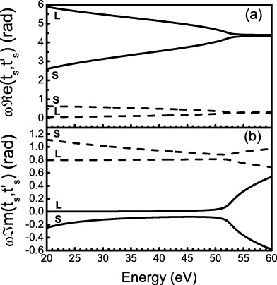
Figure 1. The real (a) and imaginary (b) parts of the ionization (dashed lines) and recombination (solid lines) times as a function of the harmonic energy calculated in argon at Up = 10.15 eV for the two first (S for short and L for long) electron trajectories. The plots for 800 and 1600 nm driving wavelength are indistinguishable.
Download figure:
Standard imageLet us now consider equation (6) in order to determine the scaling of the harmonic dipole. Since ps, A(ts) and A(t's) are constant, the dipole matrix elements dx and d*x entering equation (6) do not depend on ω. The electric field is proportional to ω, but this is compensated for by the ω dependence of  . Therefore, except for the exponential factor, one is left with the ω3/2 scaling coming from the prefactor (saddle-point integration over momenta). The spreading of the free electron wavepacket thus leads to an ω3 dependence of |x(ωq)|2. However, the imaginary part of the ionization time results in an imaginary part of the action, as shown in figure 2(b). Since the action scales as ω−1 through the time integration in equation (2), this has dramatic consequences for the yield. The real part of the action simply corresponds to a phase factor but the imaginary part gives rise to an exponential damping of the dipole strength with the driving frequency.

Figure 2. The real (a) and imaginary (b) parts of the action at 800 nm (solid lines) and 1600 nm (dashed lines) corresponding to the case of figure 1.
Download figure:
Standard imageThe imaginary part of the action in the low-frequency limit (ω → 0) can be estimated through a calculation analogous to that of the Landau–Dykhne ionization probability by a static electric field [23]. In the plateau region, this imaginary part is mostly due to times close to the (complex) ionization time, i.e. the lower bound of the integral in equation (2). Indeed, there is little trace of the tunneling effect in the recombination time, whose imaginary part is very small especially for the long trajectory, as shown in figure 1(b) [24]. We may thus restrict the integral to its lower portion close to the maximum of the laser field (between t's and θ real <ts), and make a linear approximation of the vector potential:

Making the change of variable: u = ps − E0t'' and using equation (5), one obtains

The corresponding ionization probability is

which is the well-known form of the ionization probability in the tunneling regime [22, 23, 25–27]. This result can be generalized, resulting in the following scaling for the harmonic dipole intensity:

where  is an effective Keldysh parameter calculated at the time of ionization t's [25]. The ω3 pre-exponential factor results from an increase of the wavepacket spreading along the longer trajectories induced at longer driving wavelengths. The exponential factor comes from the tunneling ionization process: the width of the potential barrier scales as 1/E0 and thus as ω at a constant Up.
The resulting change in the harmonic spectrum is illustrated in figure 3. For the long trajectory, the imaginary part of the quasi-classical action is constant below the cutoff energy, because ionization occurs very close to the peak of the laser field (see figures 1(b) and 2(b)). Spectra at different driving wavelengths thus differ from each other by a scaling factor independent of the harmonic energy in the plateau region (figure 3). This is not the case for the short trajectory contribution, for which in equation (15) the exponential factor must be replaced by the tunneling rate at the time of ionization. This rate is smaller than that for the long trajectory and changes with harmonic energy (figure 2). This explains both a larger and variable scaling factor.
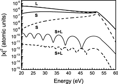
Figure 3. Harmonic spectra corresponding to the contributions of the short (S), long (L) and short + long (S + L) trajectories at 800 nm (solid line) and 1600 nm (dashed line). The S and L spectra at 1600 nm have been multiplied by a factor of 7 × 10⁵, while the S + L spectra of both 800 and 1600 nm are simply shifted for visibility.
Download figure:
Standard imageFigure 4 shows the plateau harmonic yield normalized to that at 800 nm from different theoretical methods. First we want to stress that our analysis is independent of the dipole form used (length, velocity or acceleration) [15] since we compare yields at a constant harmonic energy. The scaling from the long trajectory (red squares) is in good agreement with the scaling given by equation (15) (red solid line) for the value of γeff of 0.89 given by the ionization time reported in figure 1(a) at, e.g., 40 eV. This γ-value is very close to the one corresponding to the maximum intensity (γ = 0.88). For the short trajectory, the agreement with equation (15) is also very good: at 40 eV energy, the data (blue up triangles in figure 4) are close to the blue dashed line corresponding to γeff = 1, a value given by the field associated with the 40 eV ionization time reported in figure 1(a).
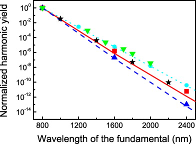
Figure 4. Normalized harmonic yield versus driving wavelength in argon for Up = 10.15 eV for different dipoles. Gaussian dipole: the saddle-point method for the long trajectories (red squares) and scaling from equation (15) with γeff = 0.89 (red solid line); the saddle-point method for the short trajectories at 40 eV harmonic energy (blue up triangles) and scaling from equation (15) with γeff = 1 (blue dashed line); numerical integration of equation (1) (black stars). Hydrogenic dipole: numerical integration of equation (1) (cyan discs) and scaling from equation (17) with γeff = 0.89 (cyan dotted line). Model argon potential: TDSE simulations (green down triangles).
Download figure:
Standard imageDefining a scaling law for the total harmonic dipole in equation (1) raises two potential problems: firstly, as shown above, the contributions of the different trajectories scale differently. Secondly, their phase difference scales as ω−1 (figure 2(a)). The quantum-path interferences [16, 28] are thus greatly modified, leading to a very different spectrum at long driving wavelength with twice as fast oscillations but reduced amplitudes, as shown in figure 3 for the sum of the short and long path contributions. In order to smooth out the undesired modulations, the scaling has to be defined over a large enough spectral bandwidth: we shall integrate the harmonic dipole in the 20–50 eV energy range. In figure 4, we report as black stars the results obtained by solving numerically equation (1) (numerical integration over both t and t', saddle point only for p) for Up = 10.15 eV, and a sin4 pulse envelope of 27 fs full-width at half-maximum, i.e. ten optical cycles at 800 nm. Note that in this calculation, return times longer than one cycle—and thus the contributions of longer trajectories—are taken into account. The corresponding ionization times are very close to the maximum of the laser field, and we thus expect that their scaling will be similar to that associated with the long path. Indeed, the scaling found is very close to the latter. The short trajectory has a more unfavorable scaling, leading to an enhanced weight of the long paths at long wavelength. We should note, however, that the SFA overestimates the contribution of the long trajectory at 800 nm [29].
When discussing equation (6), we noted that, since ps, A(ts) and A(t's) do not depend on ω, the scaling is independent of the exact form of the dipole matrix element dx. However, one should keep in mind that this is true only as long as the saddle-point integration is valid. For instance, a small variation of the scaling is observed in the results of the numerical integration on varying the α-value. This is due to the exponential form of the dipole in equation (11). For large enough α-values, i.e. in the broad Gaussian limit, the scaling becomes independent of α. More crucial are the implications of a hydrogenic dipole given by

with α = 2Ip this time [18]. Indeed, this dipole at the ionization time dx(p + A(t')) has a pole of third order at the saddle point (see equation (5)). The saddle-point integration then results in an additional prefactor that cancels the ω3 dependence in the scaling. One is then left with only the ionization rate:

as is found in [10]. Numerical integration of equation (1) for this dipole gives points (cyan discs in figure 4) that are indeed aligned on the prediction of equation (17) (cyan dotted line). In order to compare the scalings derived above, we carried out three-dimensional TDSE simulations for a flat-top ten-cycle-long laser pulse interacting with a model argon atom [30]. The data (green down triangles in figure 4) are very close with the hydrogenic dipole predictions. The dispersion in the data is presumably due to long quantum-path interferences close to channel closings that survive spectral averaging and induce a yield variation by a factor of 2–6 [16].
3. Conclusions
In summary, we have shown that, in the tunneling regime and a constant ponderomotive potential, the exponential decrease of the harmonic yield with increasing the driving wavelength is mainly due to the rapid decrease of the tunneling ionization rate. Furthermore, we have shown that the pre-exponential factor in the scaling law depends on the presence of poles in the dipole matrix element describing bound–continuum transitions. In particular, for a hydrogenic potential that has a pole of third order at the saddle point, the scaling is significantly modified and is very close to the one obtained with a model argon atom. We found that the scaling is different for the short and long path contributions to the harmonic dipole and that their relative phase is also ω-dependent: the quantum-path interferences in the harmonic spectra are thus greatly modified upon a change of the driving wavelength, allowing their precise control with attosecond accuracy.
Acknowledgments
We acknowledge enlightening discussions with W Becker and M Yu Ivanov. This research was partially supported by EU-FP7-ATTOFEL, ANR-09-BLAN-0031-02 and RTRA-Triangle-2008-045T. The work performed at OSU was supported by the USDOE/BES under contracts DE-FG02-04ER15614 and DE-FG02-06ER15833. LFD acknowledges support from the Hagenlocker chair.