


Abstract
The efficient implementation of electronic structure methods is essential for first principles modeling of molecules and solids. We present here a particularly efficient common framework for methods beyond semilocal density-functional theory (DFT), including Hartree–Fock (HF), hybrid density functionals, random-phase approximation (RPA), second-order Møller–Plesset perturbation theory (MP2) and the GW method. This computational framework allows us to use compact and accurate numeric atom-centered orbitals (NAOs), popular in many implementations of semilocal DFT, as basis functions. The essence of our framework is to employ the 'resolution of identity (RI)' technique to facilitate the treatment of both the two-electron Coulomb repulsion integrals (required in all these approaches) and the linear density-response function (required for RPA and GW). This is possible because these quantities can be expressed in terms of the products of single-particle basis functions, which can in turn be expanded in a set of auxiliary basis functions (ABFs). The construction of ABFs lies at the heart of the RI technique, and we propose here a simple prescription for constructing ABFs which can be applied regardless of whether the underlying radial functions have a specific analytical shape (e.g. Gaussian) or are numerically tabulated. We demonstrate the accuracy of our RI implementation for Gaussian and NAO basis functions, as well as the convergence behavior of our NAO basis sets for the above-mentioned methods. Benchmark results are presented for the ionization energies of 50 selected atoms and molecules from the G2 ion test set obtained with the GW and MP2 self-energy methods, and the G2-I atomization energies as well as the S22 molecular interaction energies obtained with the RPA method.
1. Introduction
Accurate quantum-mechanical predictions of the properties of molecules and materials (solids, surfaces, nano-structures, etc) from first principles play an important role in chemistry and condensed-matter research today. Of particular importance are computational approximations to the many-body Schrödinger or Dirac equations that are tractable and yet retain quantitatively reliable atomic-scale information about the system—if not for all possible materials and properties, then at least for a relevant subset.
Density-functional theory (DFT) [1, 2] is one such successful avenue. It maps the interacting many-body problem onto an effective single-particle one where the many-body complexity is hidden in the unknown exchange-correlation (XC) term, which has to be approximated in practice. Existing approximations of the XC term roughly fall into a hierarchial scheme [3]. Its local-density approximation (LDA) [2] and generalized gradient approximation (GGA) [4–7] are now well-recognized workhorses with a broad application range in computational molecular and materials science. However, several qualitative failures are well known: to name but a few, certain adsorbate geometries [8], f-electron systems [9–13] or van der Waals interactions [14–19] are not described correctly at this level of theory. Thus, there is much ongoing work to extend the reach of DFT, e.g. meta-GGAs [20–22], formalisms to include van der Waals interactions [23–28], hybrid functionals [29–34] or approaches based on the random-phase approximation (RPA) [35–42] that deal with the non-local correlations in a more systematic and non-empirical way.
Another avenue is provided by the approaches of quantum chemistry that start with Hartree–Fock (HF) theory [43, 44]. These approaches offer a systematically convergable hierarchy of methods by construction, said to reach 'gold standard' accuracy for many molecular systems at the level of coupled-cluster theory [45–47] (often taken to include singles, doubles and perturbative triples, CCSD(T) [48]). CCSD(T) theory is significantly more accurate than DFT-LDA/GGA for many molecular systems, but also significantly more costly (formally scaling as with system size). It has its own shortcomings as well. For instance, systematic, material-specific failures can occur in the cases when the underlying HF solution itself is not a good reference to start with (e.g. many open-shell systems) and a multireference extension of the approach [49] becomes necessary.

A third avenue for electronic structure calculations is the quantum Monte Carlo (QMC) method, in particular the diffusion QMC method [50, 51]. This is a stochastic approach that deals with the many-body wavefunction directly. The diffusion QMC method can often deliver high accuracy, and provide data and insight for problems that are difficult for other approaches. Its widespread use, however, is also impeded by the rather high computational cost. Moreover, the fixed-node approximation and the underlying pseudopotential approximation are known issues which limit the practical accuracy of QMC. Regarding the computational cost, the QMC methods, the algorithm of which is intrinsically parallel, are in a better position to benefit from the development of petaflop supercomputers [52].
With the successes, but also the failures or shortcomings of the aforementioned avenues, much attention is currently devoted to the construction of further, systematic and generally applicable methods or theoretical frameworks that can offer better accuracy than conventional DFT, but have lower numerical costs and are free of the limitations of CCSD(T) and QMC. Among the various possible pathways, many-body perturbation theory (MBPT) based on an efficiently attainable and trustworthy electronic reference state offers such an avenue. In particular, approaches based on the RPA, which bridge the DFT and MBPT worlds [16, 35, 36, 53], have recently enjoyed considerable attention for ground-state total-energy calculations. For electron addition and removal energies, a self-energy based approach that is consistent with the RPA total-energy treatment is Hedin's GW approximation [54]. GW is especially popular in the solid state community [55–58] and has become the method of choice for the calculation of quasiparticle band structures as measured in direct and inverse photoemission [59–61].
Although RPA and GW are receiving much attention in the community today, the systematic investigation of diagrammatic perturbation theory from first principles for real materials is only just beginning. Its full promise lies in the fact that it is intermediate in cost between DFT and coupled-cluster theories and applicable in practice to molecular and bulk materials alike—including open-shell systems and metals.
Besides the more generally applicable RPA and GW approaches, another correlation method that is widely used in computational chemistry is second-order Møller–Plesset perturbation theory (MP2) [44, 62], which belongs to the category of HF-based quantum chemistry approaches mentioned above. MP2 does not reach the CCSD(T) accuracy, but its more favorable computational scaling makes it applicable to larger system sizes. In analogy to the GW self-energy, an MP2 self-energy approach [44, 63] that is compatible with the MP2 total energy is possible as well. As will be demonstrated more clearly in the next section, RPA, GW and MP2 (both total and self-energy) are related approaches both diagramatically and numerically. The development of numerical frameworks that enable the implementation of all these approaches on an equal footing with high numerical efficiency and accuracy is thus highly desirable.
In this work, we describe the underpinnings of such a unified numerical framework that is promising to boost the efficiency of all the above-mentioned methods, by allowing for their implementation with compact and efficient NAO basis sets. Our specific implementation is based on the 'Fritz Haber Institute ab initio molecular simulations' (FHI-aims) [64] program package. While we make reference to FHI-aims basis sets throughout much of this work, the numerical foundation presented here is general: applicable to any other type of atom-centered basis set. We note that many production-quality implementations of hybrid functionals, HF and MBPT are based on analytical basis functions such as Gaussian-type orbitals (GTOs) or plane waves, and typically rely on pseudopotential-type approaches. In contrast, we here aim for an all-electron, full-potential treatment with NAO basis sets that does not sacrifice accuracy compared to the alternatives.
For DFT-LDA/GGA, NAOs are well established and can be found in several implementations [64–70]. This is, however, not the case for HF and the MBPT approaches we are going to address in this paper. Specifically, we will present in the following:
- (i)An atom-centered resolution of identity (RI) framework analogous to what is pursued in quantum chemical methods [71–78]. This framework allows us to reduce all four-center two-electron Coulomb integrals to precomputed three- and two-center integrals. Our scheme differs from the quantum chemistry approach [77, 78] in the auxiliary basis set construction, which is essential for retaining the flexibility to work with any atom-centered basis function shape, rather than being restricted to analytical shapes only.
- (ii)An assessment of the accuracy of the NAO basis sets used for normal LDA/GGA calculations in FHI-aims, and intended to be transferable regardless of the specific underlying materials or functionals, for HF, MP2, hybrid functionals, RPA and GW.
Reference is made throughout this work to relevant work by other groups in electronic-structure theory.
This paper demonstrates our approach for molecular (non-periodic) systems and makes extensive use of established GTO basis sets for comparison and reference purposes. In addition, we provide benchmark GW vertical (geometry of the ionized molecule not relaxed) ionization energies (IEs) for a subset of the G2 ion test set [79], and benchmark binding energies (RPA) for the G2-I and S22 molecular test sets [80]. We restrict ourselves to algorithms that have standard scaling with system size ( for HF, for MP2, etc). Regarding total energy differences we restrict ourselves to a discussion of counterpoise-corrected [81] results when assessing the accuracy of MBPT methods that utilize the full (also unoccupied) spectrum.


In the following, we first recapitulate the HF, MP2, RPA and GW methods and highlight the structural similarity and difference of the three correlation methods (section 2). We then introduce the basics of RI and the RI formulation of the above methods (section 3). Our own RI prescription and its accuracy is the subject of section 4. Section 5 demonstrates the overall accuracy of our approach with NAO basis sets for a variety of test systems for HF, MP2, hybrid density functionals, RPA and GW. The benchmark results for a subset of the G2 and S22 molecular test sets using our approaches are presented in section 6. Finally, we conclude our paper in section 7.
2. Theoretical framework: Hartree–Fock (HF), hybrid density functionals, second-order Møller–Plesset (MP2) perturbation theory, random-phase approximation (RPA) and GW
2.1. Many-electron Hamiltonian and many-body perturbation theory
HF theory, hybrid density functionals and MBPT (MP2, RPA and GW) are all approximate ways to solve the interacting many-electron Hamiltonian

where Ne is the number of electrons that interact via the Coulomb interaction veeij ≡ 1/|ri − rj|, and vexti ≡ vext(ri) is a local, multiplicative external potential, usually due to the nuclei. Hartree atomic units are used throughout this paper. The numerical cost for an exact solution of the Hamiltonian (1) scales exponentially with system size (the number of electrons). The systems for which such a solution is possible are thus heavily restricted in size. In general, accurate approximations are needed. The most common approximations first resort to the solution of a mean-field, non-interacting Hamiltonian that yields an approximate ground-state wave function |Φ0〉:


The '(0)' in E(0)0 implies the fact that this is the ground-state energy of the mean-field Hamiltonian. A suitable should be solvable with relative ease. |Φ0〉 is a single Slater determinant formed from the lowest Ne single-particle spin-orbitals determined by


where σ denotes the spin index and is the effective single-particle Hamiltonian noted in the brackets of (2). The form of (2)–(3) is, of course, precisely that of the Kohn–Sham (KS) DFT (with a local mean-field potential vMFi), or of HF theory and hybrid functionals (with a non-local mean-field potential vMFi).

The purpose of starting with (1)–(3) is to establish our notation for the following sections and to distinguish between
- (the many-electron Hamiltonian),
- the mean-field Hamiltonian , the solutions of which are many-electron wave functions given by single Slater determinants and define an excited-state spectrum of their own (obviously not the same as that of ),
- the effective single-particle Hamiltonian , which generates the single-particle orbitals ψnσ and orbital energies
 nσ.
nσ.


In MBPT, one starts from and the associated eigenenergies and eigenfunctions to systematically approximate the properties of , e.g. its true ground-state energy E0 in MP2 or RPA or its single-particle excitations in GW. The interacting many-electron Hamiltonian is partitioned into a mean-field Hamiltonian as given by (2) and an interaction term ,


In the remainder of this section we collect the basic formulae that define the mean-field Hamiltonians, perturbation theory for ground-state properties (MP2, RPA) and perturbation theory for excited states (electron addition and removal energies, through either GW or MP2 self-energies). From a numerical point of view, the underpinning of all these methods is the same: an efficient, accurate basis set prescription, and an efficient expansion of the two-electron Coulomb operator, which is the primary focus of this paper.
2.2. Mean-field Hamiltonians of HF or density functional theory (DFT)
In HF theory the ground-state wave function of the Hamiltonian in (1) is approximated by a single Slater determinant |Φ0〉 and E(0)0 is obtained by a variational optimization, leading to

Here denotes the HF single-particle Hamiltonian, and vh(r) is the Hartree potential,


with the electron density

and Σxσ is the non-local, exact-exchange potential

Equations (5)–(8) form a set of nonlinear equations that have to be solved iteratively. vh(r) and Σxσ(r,r') together yield the HF potential vHF, a special case of the mean-field potential vMFi in (2) and (4). The HF wavefunction |Φ0〉 is given by the Slater determinant formed by the Ne spin-orbitals ψnσ with lowest energies nσ.
At self-consistency, the HF total energy is

where the Hartree energy Eh and exact-exchange energy Ex are given, respectively, by

In general, the single-particle spin-orbitals ψnσ(r) are expanded in terms of a set of basis functions {φi(r)}

where cinσ are the expansion coefficients. In terms of these basis functions, the HF effective potential can be expressed in a matrix form

where in particular the exact-exchange matrix is given by

In (12) Dkl,σ is the density matrix

and (ij|kl) is the shorthand notation of quantum chemistry for four-center two-electron integrals

Very similar equations arise in KS-DFT with a local vMFi, or in the generalized KS scheme [82] with a fraction of Σxσ(r,r') in the potential. In principle, the exact KS-DFT would yield the exact many-electron ground-state energy E0 and ground-state density n0(r). In practice, the XC energy functional and potential have to be approximated. The effective single-particle orbitals either from HF or from approximate KS-DFT are convenient starting points for MBPT.
2.3. Perturbation theory for the many-electron ground-state energy: MP2
Assuming that is benign and can be treated as a perturbation on top of , the ground-state energy for the interacting system can be obtained using the Rayleigh–Schrödinger perturbation theory (RSPT) or more precisely the Brueckner–Goldstone perturbation theory [83, 84]. According to the Goldstone theorem [84], in a diagrammatic expansion of the ground-state total energy, only the 'linked' diagrams need to be taken into account. This guarantees the size-extensivity of the theory, i.e. the total energy scales correctly with the system size. The Møller–Plesset (MP) perturbation theory is a special case of RSPT [62], where the reference Hamiltonian is the HF Hamiltonian . Terminating the expansion at second order gives the MP2 theory, in which the (second-order) correlation energy is given by


Here Φk are the Slater determinants representing the excited states of , and E(0)k are the corresponding excited-state energies. is given by (4) with vMF = vHF. Among all possible excited-state configurations Φk, only double excitations contribute in (15). This is because singly excited Φk do not couple to the ground state Φ0 (Brillouin's theorem [44] for the HF reference), whereas even-higher-excited configurations (triples, quadruples, etc) do not contribute due to the two-particle nature of the operator H'. As such, equation (15) can be expressed in terms of single-particle spin-orbitals,


where (ma,σ|nb,σ') are two-electron Coulomb repulsion integrals for molecular orbitals

The two terms in (16) correspond to the second-order Coulomb (direct) and second-order exchange energy, respectively.
2.4. Perturbation theory for the many-electron ground-state energy: RPA
MP2 corresponds to the second-order term in a perturbation theory where the perturbation expansion is essentially based on the bare Coulomb operator (with the HF effective potential subtracted). As such, the MP2 correlation energy diverges for the 3-dimensional homogeneous electron gas and metals with zero direct energy gap. To overcome this problem in the framework of MBPT it is essential to sum up the diverging terms in the perturbation series to infinite order. One such example which has gained considerable popularity recently [38, 39, 85–98] is the RPA [16, 35, 36, 53, 99] that in the context of MBPT corresponds to an infinite summation of 'ring' diagrams. The choice of the non-interacting reference Hamiltonian can be, e.g., HF or DFT with any desired XC functional.

Apart from the diagrammatic representation, RPA can also be formulated in other ways, e.g. as the simplest time-dependent Hartree approximation in the context of the adiabatic-connection fluctuation-dissipation theorem [16, 53, 99] or as a subclass of terms in coupled-cluster theory with double excitations [87]. In the context of DFT [53], RPA calculations can be performed self-consistently by means of the OEP approach [100–103].
In close-packed notation, the RPA correlation energy (cRPA) can be expressed in terms of the RPA dielectric function ε, or alternatively the non-interacting density response function χ0 on the imaginary frequency axis

The real-space (Adler–Wiser [104, 105]) representation of χ0 reads

where c.c. denotes 'complex conjugate', and ψn(r) and n are single-particle orbitals and orbital energies as implied by (3). The RPA dielectric function ε is linked to χ0 through

Using (17) and (19), the lowest-order term in (18) can be expressed as

Higher-order terms in (18) follow analogously. There is thus a straightforward path to compute χ0 and hence the RPA correlation energy once the selected non-interacting reference state is solved. In practice, the RPA correlation energy is always combined with the exact-exchange energy (EX) in (9), henceforth denoted as (EX + cRPA), but evaluated with the same single-particle orbitals as used in ERPAc. The choice of input orbitals will in the following be marked by (EX + cRPA)@MF, where MF specifies the mean-field approach used to compute the single-particle orbitals. The application of EX + cRPA to various realistic systems, as well as the development of schemes that go beyond simple EX + cRPA, is an active field [38–40, 85–89, 91–98, 106–109]. For instance, when the so-called single-excitation and second-order screened exchange contributions [90, 110] are added to EX + cRPA, the resulting accuracy is impressive [40, 41].
2.5. Perturbation theory for electron addition or removal energies: GW or MP2
Besides ground-state energies, one is often interested in the properties of electronically excited states. Part of this information is, in principle, accessible by taking the difference in the total energies of the N-electron system and the N ± 1-electron systems using approaches discussed above. In practice, this approach mainly works for computing core-level excitations and/or the first IE and electron affinity for (small) finite systems. In contrast, Green function techniques are more convenient and powerful in dealing with electronic excitations in general. The basic theory of Green functions is well documented in textbooks [111, 112]. Here we collect the contextual equations based on which practical approximations can be introduced.
The single-particle Green function of an interacting many-electron system is defined as

where denotes the interacting ground-state wave function of an N-electron system (solution to (1)). and are field operators in the Heisenberg picture that annihilate and create an electron at space–time point (r,t) and (r',t'), respectively. is the time-ordering operator. The Green function G(r,t;r',t') measures the probability amplitude of a hole created at (r, t) propagating to (r',t') for t < t', or an electron added at (r',t') propagating to (r, t) for t > t'. The poles of its Fourier transform, G(r,r',ω), correspond to the single-particle excitation energies as measured, for example, in direct and inverse photoemission experiments.


For Hamiltonians with a time-independent external potential, as considered in this paper, the Green function depends only on the difference between t and t', G(r,t;r',t') = G(r,r';t − t'). Its Fourier transform gives the frequency-dependent Green function G(r,r';ω) that satisfies the Dyson equation

Here vh(r) is the electrostatic Hartree potential defined in (6) and Σ(r,r'',ω) is the dynamical, non-local, complex self-energy that contains all the many-body XC effects.
G(r,r';ω) and Σ(r,r';ω) for many-body interacting systems can, in principle, be obtained using the diagrammatic Feynman–Dyson perturbation theory. The perturbation series is built on a non-interacting Green function G0(r,r',ω) that corresponds to the non-interacting single-particle Hamiltonian . With single-particle orbitals ψnσ(r) and orbital energies nσ of , one has


where F is the Fermi energy and η a positive infinitesimal. For a given G0, corrections to the single-particle excitation energies can be computed from approximate perturbative expansions of Σ(r,r';ω). Examples are the GW method and the second-order approximations discussed below.
In the GW approximation proposed by Hedin [54], the self-energy assumes the form

Here W is the screened Coulomb potential at the RPA level

with the dynamical dielectric function ε as defined in (19) and (20), but on the real frequency axis with iω replaced by ω + iη (η → 0+).
In practice, one-shot perturbative GW calculations (often referred to as G0W0) based on a fixed, non-interacting reference state (DFT with popular functionals or HF) are often performed. With χ0 computed from the non-interacting Green function in (24), the ensuing W can be expanded in powers of χ0v:

The GW approximation can thus be regarded as an infinite series in the bare Coulomb potential v, or alternatively, as is obvious from (25), as first-order perturbation in terms of the screened Coulomb potential W.
Once the G0W0 self-energy is obtained from (25), the corrections to the single-particle orbital energies are given by

where the XC part vxc of the reference mean-field potential has to be subtracted. Equation (28) approximates the quasiparticle wavefunctions with the single-particle orbitals of the reference state. This is often justified, but may break down in certain cases [113–118].
Rewriting the diagonal elements of the G0W0 self-energy on the imaginary frequency axis in terms of four-center Coulomb integrals, we obtain

where G0mσ(iω) = 1/(iω + F − mσ) and

This expression can be analytically continued to the real-frequency axis using the Padé approximation or a two-pole model [119].
The G0W0 approach, as a highly popular choice for quasiparticle excitation calculations, in particular for solids [59–61, 120, 121], is akin to the RPA approach for computing the ground-state correlation energy. Similarly, one can also introduce a second-order perturbation theory for the self-energy [44] consistent with the MP2 correlation energy. Based on the HF non-interacting Green function (equation (24) with HF orbitals), the second-order self-energy can be expressed as

Here for notational simplicity, we have used 1 = (r1,t1) and v(1,2) = v(r1 − r2)δ(t1,t2). After integrating out the internal (spatial and time) coordinates in (31), the final expression for Σ(2) (in the frequency domain) within the HF molecular orbital basis is given by

where θ(x) is the Heaviside step function and η → 0+. Again, the two lines in (32) correspond to correlations arising from the second-order direct and second-order exchange interaction, respectively. With this self-energy single-particle excitation energies—here denoted by MP2 quasiparticle energies—can be obtained by adding a correction to the HF orbital energies

Similar to the MP2 correlation energy, the quality of the MP2 self-energy as given by (32) will deteriorate as the single-particle energy gap shrinks.
By means of the Dyson equation G = G0 + G0ΣG, self-consistent Green functions and self-energies could be obtained. The advantage is that the self-consistent Green function will then be independent of G0 and satisfies particle number, momentum and energy conservation [122, 123]. For an in-depth discussion, see [124, 125] and references therein.
3. Resolution of identity for HF, MP2, RPA and GW
3.1. Background
In this section we present the basic RI formalism: the auxiliary basis sets, different variants of RI and the working equations for HF, hybrid density functionals, MP2, RPA and GW. Similar accounts have been given in the literature on one or the other of the above methods; see [76–78, 126–129]. Our aim here is to lay out a complete description of all necessary specifics in one consistent notation that will allow us to present our own developments (the next sections) in a self-contained way.
The common ingredient of all methods introduced in section 2 (HF, hybrid functionals, MP2, RPA and GW) is the four-orbital Coulomb integrals

where (ij|kl) are the two-electron integrals in a basis set representation as defined in (14), and cimσ are the eigen-coefficients for the molecular orbitals. Computing (and possibly storing) these four-center two-electron integrals can be a major bottleneck for approaches beyond LDA and GGAs.
For analytical GTOs, algorithms have been developed to handle (mn,σ|ab,σ') integrals efficiently and on the fly [130, 131]. More general NAOs, however, are not amenable to such algorithms. In the context of HF, we note that RI is not the only technique available to deal with the four-center integrals: making use of the translational properties of spherical harmonics, Talman and others have developed the techniques based on multipole expansions of basis functions [132–135]. Multi-center NAO integrals can then be treated partially analytically. Alternatively, efficient Poisson solvers [136] have recently been used to enable direct NAO HF calculations through four-center integrals for simple systems [133, 136]. Finally, another different numerical route (based on expanding orbital products directly) has been adopted along the line of time-dependent DFT in the linear-response framework [137]. RI is, however, most successful at reducing the computational load compared to direct four-center integral-based methods, most prominently for MP2 in quantum chemistry [77], which is why we pursue this route here.
3.2. Auxiliary basis
The RI or synonymously the density fitting technique [71–78] amounts to representing pair products of atomic basis functions φi(r)φj(r) in terms of auxiliary basis functions (ABFs),

μ = 1,2,...,Naux labels the ABFs {Pμ}, Cμij are the expansion coefficients, and ρij(r) and here denote pair products of basis functions and their approximate expansion in ABFs. The evaluation of the four-center integrals in (14) then reduces to


To determine the expansion coefficients Cμij, three-center integrals involving the ABFs and the pair products of the NAOs are required. Thus the expensive (both in time and memory, if there is a need to pre-compute numerical matrix elements) four-center integrals reduce to the much cheaper three-center and two-center ones in RI. The key reason for the success of RI lies in the fact that the set of all possible pair products {φi(r)·φj(r)}, as a set of basis functions in three-dimensional (3D) function space, is heavily linearly dependent. Their number scales quadratically with system size, while a non-redundant basis set that expands the same 3D space should scale linearly with system size. For example, the non-interacting response function χ0 in (19), as well as the screened Coulomb interaction W in (26), is written in terms of orbital pair products and hence can be represented in terms of the ABFs. As will be shown below, this naturally leads to an RI implementation for RPA and GW.
Next we will present RI formulations for all pertinent methods in this paper before presenting our specific choice for the ABFs.
3.3. Metric and variational principle in resolution of identity (RI)
For a given set of ABFs {Pμ(r)}, the way to determine the expansion coefficients Cμij is not unique. Different variational procedures give rise to different versions of RI and different working equations for computing the Cμij [71–78].
The expansion error of basis products in terms of the ABFs (equation (35)) is

One choice for the construction of the expansion coefficients Cμij is to minimize the residual δρij(r). A simple least-square fit amounts to minimizing the norm of the residual, , and yields


where

and

Combining (36) and (39), one arrives at the following approximation to the four-center Coulomb integrals:

In the literature, equation (42) is therefore referred to as the 'SVS' version [75] of RI ('RI-SVS' in the following) because of the appearance of the inverse S before and after the V matrix in (42).
A better criterion for obtaining Cμij is to directly minimize the RI error of the four-center integrals themselves,

As shown by Whitten [72], δIij,kl has an upper bound:

The minimization of δIij,kl can thus be achieved by independently minimizing δUij = (δρij|δρij) and δUkl = (δρkl|δρkl)—the self-repulsion of the basis pair density residuals. Minimizing δUij with respect to Cμij leads to [72–75]

where

and the Coulomb matrix V is defined in (37). Combining (36) and (45) one obtains the following decomposition of the four-center ERIs:

Equation (47) is based on the global Coulomb metric and corresponds to the 'RI-V' method [75] mentioned earlier. 'RI-V' has long been known to be superior to 'RI-SVS' in the quantum chemistry community [72–75]. This can be most easily seen by inspecting the error introduced in the self-Coulomb repulsion of the NAO pairs,

In the RI-V approximation, the first term in the above equation vanishes, and the non-zero contribution comes only from the second order of δρij. This can be readily verified as follows:

where (35) and particularly (45) have been used. In contrast, in RI-SVS the term linear in δρ is non-zero and represents the dominating contribution to the total error.
Our preferred flavor of RI is therefore RI-V, based on the Coulomb metric [72–78], on which all working equations for HF and other approaches presented further down in this section are based. Before proceeding we reiterate that RI-V continues to be the de facto standard in quantum chemical calculations, due to its well-established accuracy and reliability [77, 78].
That said, the long-range nature of the Coulomb interaction does present a bottleneck for implementations that scale better than the textbook standard (e.g. better than O(N4) for HF). In order to avoid delocalizing each localized two-center basis function product entirely across the system through Cμij, more localized approaches would be desirable. Research into better-scaling RI expansions that retain at least most of the accuracy of the Coulomb metric is thus an active field, for example by Cholesky decomposition techniques or an explicitly local treatment of the expansion of each product (see, e.g., [138–145] for details). In fact, a promising Coulomb-metric based, yet localized, variant of RI has been implemented in FHI-aims. In this approach products of orbital basis functions are only expanded into ABFs centered at the two atoms at which the orbital basis functions are centered, but the appropriate RI sub-matrices are still treated by the Coulomb metric [146]. As expected, the error cancellation in this approach is not as good as that in full RI-V, but—for HF and hybrid functionals—certainly more than an order of magnitude better than in RI-SVS, creating a competitive alternative for the cases when RI-V is prohibitive. More details go beyond the scope of this paper and will be presented in a forthcoming publication [147].
3.4. HF and hybrid functionals
The key quantity for HF and hybrid functionals is the exact-exchange matrix—the representation of the non-local exact-exchange potential (equation (8)) in terms of basis functions as given in (12). Its RI-V expansion follows by inserting (47) into (12):

where

Σxij,σ must thus be recomputed for each iteration within the self-consistent field (scf) loop. The required floating point operations scale as N3b·Naux, where Nb is the number of regular single-particle basis functions. The transformation matrix Mμik, on the other hand, is constructed only once (prior to the scf loop), requiring N2b·N2aux operations.
The numerical efficiency can be further improved by inserting the expression for the density matrix (13) into (49):

The formal scaling in (51) is now Nocc·Nb2·Naux, with Nocc being the number of occupied orbitals, and is thus improved by a factor Nb/Nocc (typically 5–10). Once the exact-exchange matrix is obtained, the EX follows through

For a variety of physical problems, combining HF exchange with semi-local exchange and correlation of the GGA type gives much better results than with pure HF or pure GGAs [29]. Various flavors of these so-called hybrid functionals exist in the literature. The simplest one-parameter functionals are of the following form:

In the PBE0 hybrid functional [30], the GGA is taken to be PBE, and the mixing parameter α is set to 1/4. Naturally, the computational cost of hybrid functionals is dominated by the HF exchange. Once the HF exchange is implemented, it is straightforward to also perform hybrid functional calculations.
3.5. MP2 (total energy and self-energy)
To compute the MP2 correlation energy in (16) and the MP2 self-energy in (32) using the RI technique, the MO-based four-orbital two-electron Coulomb integrals are decomposed as follows:

The three-orbital integrals can be evaluated by

following (34), (47) and (50). Plugging (54) into (16), one obtains the RI-V version of the MP2 correlation energy

In practice, one first transforms the atomic orbital-based integrals Mμij to MO-based ones Oμma,σ. The transformation scales formally as Nocc·N2b·Naux and the summation in (56) as N2occ·(Nb − Nocc)2·Naux. Like in HF, the scaling exponent is therefore not reduced by RI-V. However, the prefactor in RI-MP2 is one to two orders of magnitude smaller than in full MP2.

The computation of the MP2 self-energy at each frequency point proceeds analogous to that of the correlation energy. In our implementation, we first calculate the MP2 self-energy on the imaginary frequency axis, Σ(2)mn,iσ, and then continue analytically to the real frequency axis using either a 'two-pole' model [119] or the Padé approximation. Both approaches have been implemented in FHI-aims and can be used to cross-check each other to guarantee the reliability of the final results.
3.6. RPA and GW
To derive the working equations for the RPA correlation energy and the GW self-energy in the RI approximation, it is illuminating to first consider the RI decomposition of Tr . Combining (19) and (54) we obtain
![$\left [\chi ^0(\mathrm {i}\omega)v\right ]$](https://content.cld.iop.org/journals/1367-2630/14/5/053020/revision1/nj418651ieqn33.gif)

where Oμma,σ is given by (55). Next we introduce an auxiliary quantity Π(iω):

which allows us to write

Thus the matrix Π can be regarded as the matrix representation of the composite quantity v1/2χ0(iω)v1/2 using the ABFs. It is then easy to see that the RPA correlation energy (18) can be computed as

using the general property Tr for any matrix A. This is very convenient since all matrix operations in (60) occur within the compressed space of ABFs and the computational effort is therefore significantly reduced.
![$\left [ \ln (A)\right ]=\ln \left [{\mathrm { det}}(A)\right ]$](https://content.cld.iop.org/journals/1367-2630/14/5/053020/revision1/nj418651ieqn34.gif)
In practice, we first construct the auxiliary quantity Π(iω) (equation (58)) on a suitable imaginary frequency grid where we use a modified Gauss–Legendre grid (see appendix C for further details) with typically 20–40 frequency points. For a fixed frequency grid size, the number of required operations is proportional to Nocc·Nunocc·N2aux (Nunocc is the number of unoccupied orbitals using the full spectrum of our Hamiltonian matrix). The next step is to compute the determinant of the matrix 1 − Π(iω) as well as the trace of Π(iω). What remains is a simple integration over the imaginary frequency axis. Thus our RI-RPA implementation is dominated by the step in (58) that has a formal scaling. An -scaling algorithm of RI-RPA was recently derived from a different perspective [129], based on the plasmonic formulation of RPA correlation energy [107] and a transformation analogous to the Casimir–Polder integral [148]. An even better scaling can be achieved by taking advantage of the sparsity of the matrices involved [145].


Finally, we come to the RI-V formalism for GW. To make (30) tractable, we expand the screened Coulomb interaction W(iω) in terms of the ABFs. Using (27) and Π(iω) = v1/2χ0(iω)v1/2, we obtain

To apply the RI-decomposition to (30), we expand

where (10) and (35) are used. Combining (30), (50), (55) and (61) gives

Inserting (62) into (29), one finally arrives at the RI version of the G0W0 self-energy

As stated above for the MP2 self-energy, the expression is analytically continued to the real-frequency axis before the quasiparticle energies are computed by means of (28).
4. Atom-centered auxiliary basis for all-electron NAO calculations
4.1. Orbital basis set definitions
For the practical implementation, all the aforementioned objects (wave functions, effective single-particle orbitals, Green function, response function, screened Coulomb interaction, etc) are expanded either in a single-particle basis set or in an auxiliary basis set. We first summarize the nomenclature used for our NAO basis sets [64] before defining a suitable auxiliary basis prescription for RI in the next subsections.
NAO basis sets {φi(r)} to expand the single-particle spin orbitals ψnσ(r) (equation (10)) are of the general form

us(a)lκ is a radial function centered at atom a, and is a spherical harmonic. The index s(a) denotes the element species s for an atom a, and κ enumerates the different radial functions for a given species s and an angular momentum l. The unit vector refers to the position Ra of atom a. The basis index i thus combines a, κ, l and m.


For numerical convenience and without losing generality, we use real-valued basis functions, meaning that the Ylm(Ω) denote the real (for m = 0,...,l) and the imaginary part (for m = −l,...,−1) of complex spherical harmonics. For NAOs, us(a)lκ(r) need not adhere to any particular analytic shape, but are tabulated functions (in practice, tabulated on a dense logarithmic grid and evaluated in between by cubic splines). Of course, Gaussian, Slater-type or even muffin-tin orbital basis sets are all special cases of the generic shape (64). All algorithms in this paper could be used for them. In fact, we employ the Dunning GTO basis sets (see [149, 150] and references therein) for comparison throughout this paper.
Our own implementation, FHI-aims, [64] provides hierarchical sets of all-electron NAO basis functions. The hierarchy starts from the minimal basis composed of the radial functions for all core and valence electrons of the free atoms. Additional groups of basis functions, which we call tiers (quality levels), can be added for increasing accuracy (for brevity, the notation is minimal, tier 1, tier 2, etc). Each higher level includes the lower level. In practice, this hierarchy defines a recipe for systematic, variational convergence down to meV per atom accuracy for total energies in LDA and GGA calculations. The minimal basis (atomic core and valence radial functions) is different for different functionals, but one could also use, e.g., LDA minimal basis functions for calculations using other functionals if their minimal basis functions are not available. Below we discuss this possibility for HF.
To give one specific example, consider the nitrogen atom (this case and more are spelled out in detail in table 1 of [64]). There are five minimal basis functions, of 1s, 2s and 2p orbital character, respectively. In shorthand notation, we denote the number of radial functions for given angular momenta by (2s1p) (two s-type radial functions and one p-type radial function). At the tier 1 basis level, one s, p and d function is added to give a total of 14 basis functions (3s2p1d). There are 39 basis functions (4s3p2d1f1g) in tier 2, 55 (5s4p3d2f1g) in tier 3 and 80 (6s5p4d3f2g) in tier 4.
4.2. Construction of the auxiliary basis
In the past, different communities have adopted different strategies for building auxiliary basis sets. For the GTO-based RI-MP2 method [77], which is widely used in the quantum chemistry community, a variational procedure has been used to generate optimal Gaussian-type atom-centered ABF sets. In the condensed matter community a so-called 'product basis' has been employed in the context of all-electron GW implementations based on the linearized muffin-tin orbital (LMTO) and/or augmented plane-wave (LAPW) method [151] to represent the response function and the Coulomb potential within the muffin-tin spheres [126, 127, 152]. Finally, it is even possible to generate ABFs only implicitly, by identifying the 'dominant directions' in the orbital product space through singular value decomposition (SVD) [144, 145, 153]. As will be illustrated below, our procedure to construct the ABFs combines features from both communities. Formally it is similar to the 'product basis' construction in the GW community, but instead of the simple overlap metric the Coulomb metric is used to remove the linear dependence of the 'products' of the single-particle basis functions and to build all the matrices required for the electronic structure schemes in this paper.
Our procedure employs numeric atom-centered ABFs whereby the infrastructure that is already available to treat the NAO orbital basis sets can be utilized in many respects. Specifically, the ABFs are chosen as

just like for the one-particle NAO basis functions in (64), but of course with different radial functions. To distinguish the ABFs from the NAO basis functions, we denote the radial functions of the ABFs by ξs(a)lκ.
The auxiliary basis should primarily expand products of basis functions centered on the same atom exactly, but at the same time be sufficiently flexible to expand all other two-center basis function products with a negligible error. In contrast to the ABFs used in the GTO-based RI-MP2 method [77], in our case the construction of ABFs follows from the definition of the orbital basis set. At each level of NAO basis, one can generate a corresponding ABF set, denoted by aux_min, aux_tier 1, aux_tier 2, etc. We achieve this objective as follows:
- (i)For each atomic species (element) s and for each l below a limit lmaxs, we form all possible 'on-site' pair products of atomic radial functions . The allowed values of l are given by the possible multiples of the spherical harmonics associated with the orbital basis functions corresponding to usk1l1 and usk2l2, i.e. |l1 − l2| ⩽ l ⩽ |l1 + l2|.
- (ii)Even for relatively small orbital basis sets, the number of resulting auxiliary radial functions is large. They are non-orthogonal and heavily linear dependent. We can thus use a Gram–Schmidt-like procedure (separately for each s and l) to keep only radial function components ξslκ(r) that are not essentially represented by others, with a threshold for the remaining norm εorth, below which a given radial function can be filtered out. In doing so, the Coulomb metric is used in the orthogonalization procedure. The result is a much smaller set of linearly independent, orthonormalized radial functions {ξslκ(r)} that expand the required function space.
- (iii)The radial functions {ξs(a),lκ} are multiplied by the spherical harmonics as in (65).
- (iv)The resulting {Pμ(r)} are orthonormal if they are centered on the same atom, but not if situated on different atoms. Since we use large ABF sets, linear dependences could also arise between different atomic centers, allowing us to further reduce the ABF space through SVD of the applied metric (S in the case of RI-SVS, V in the case of RI-V). For the molecule-wide SVD we use a second threshold εsvd, which is not the same as the on-site Gram–Schmidt threshold εorth.


For a given set of NAOs, the number of the corresponding ABFs depends on the angular momentum limit lmaxs in step 1 and the Gram–Schmidt orthonormalization threshold εorth and to a small extent on εsvd. For RI-V, as documented in the literature [78] and demonstrated later in this paper (section 4.5), it is sufficient to keep lmaxs just one higher than the highest angular momentum of the one-electron NAOs. Usually εorth = 10−2 or 10−3 suffices for calculations of energy differences. Nevertheless, both lmaxs and εorth can be treated as explicit convergence parameters if needed. In practice, we keep εsvd as small as possible, typically 10−4 or 10−5, only large enough to guarantee the absence of numerical instabilities through an ill-conditioned auxiliary basis. The resulting auxiliary basis size is typically 3–6 times that of the NAO basis. This is still a considerable size and could be reduced by introducing optimized ABF sets as is sometimes done for GTOs. On the other hand, it is the size and quality of our auxiliary basis that guarantees low expansion errors for RI-V, as we will show in our benchmark calculations below. We therefore prefer to keep the safety margins of our ABFs to minimize the expansion errors, bearing in mind that the regular orbital basis introduces expansion errors that are always present.
4.3. Numerical integral evaluation
With a prescription to construct ABFs at hand, we need to compute the overlap integrals Cμij, defined in (39) for RI-SVS or in (45) for RI-V, respectively. We also need their Coulomb matrix given by (37) in general, and additionally the 'normal' overlap matrix Sμν given by (41) in RI-SVS. Having efficient algorithms for these tasks is very important, but since many pieces of our eventual implementation exist in the literature, here we give only a brief summary; see the separate appendices for details.
Since our auxiliary basis set {Pμ} is atom-centered, we obtain the Coulomb potential Qμ(r) of each Pμ(r) by a one-dimensional integration for a single multipole (appendix A.1). The required three-center integrals

are carried out by standard overlapping atom-centered grids as used in many quantum-chemical codes for the XC matrix in DFT [64, 65, 154, 155]; see appendix A.2. The same strategy works for two-center integrals

As an alternative, we have also implemented two-center integrals following the ideas developed by Talman [133, 134], which are described in appendices A.3 and A.4. In summary, we thus have accurate matrix elements at hand that are used for the remainder of this work.
4.4. Accuracy of the auxiliary basis: expansion of a single product
In this section we examine the quality of our prescription for generating the ABFs as described in section 4.2. Our procedure guarantees that the ABFs accurately represent the 'on-site' products of the NAO basis pairs by construction, but it is not a priori clear how the 'off-site' pairs are represented. The purpose of this section is to demonstrate the quality of our ABFs to represent the 'off-site' pairs.
In the left panels of figure 1 we plot ρ2s−2px(r) for a simple N2 molecule at the equilibrium bonding distance (d = 1.1 Å)—the product of the atomic 2s function from the left atom and the atomic 2px function from the right atom. We compare this directly taken product to its ABF expansions, both in RI-SVS (equation (39)) and in RI-V (equation (45)). The particular product ρ2s−2px(r) is part of the minimal basis of free-atom-like valence radial functions. As we increase the orbital basis set (adding tier 1, tier 2, etc), the exact product remains the same, whereas its ABF expansion will successively improve, since the auxiliary basis set is implicitly defined through the underlying orbital basis. Three different levels of ABF sets are shown (aux_min, aux_tier 1, aux_tier 2 from the top to bottom panels). The onsite threshold εorth is set to 10−2, and the global SVD threshold εsvd is set to 10−4, yielding 28, 133 and 355 ABFs, respectively. In the right panels of figure 1, the corresponding δρ2s−2px(r)—the deviations of the ABF expansions from the reference curve—are plotted. One can clearly see two trends: firstly, the quality of the ABF expansion improves as the number of ABFs increases. Secondly, at the same level of ABF, the absolute deviation of the RI-V expansion is larger than the RI-SVS expansion. This is an expected behavior for the simple pair product: RI-V is designed to minimize the error of the Coulomb integral; see section 3.3. In either method, the remaining expansion errors are centered around the nucleus, leading to a relatively small error in overall energies (in the 3D integrations, the integration weight r2 dr is small).

Figure 1. Left panels: the product of the atomic 2s and 2px functions centered, respectively, on the two atoms in a N2 molecule along the bonding direction, and its approximate behaviors from the RI-SVS and RI-V expansions for three hierarchical levels of ABFs (from aux_min to aux_tier 2). Right panels: the corresponding deviations of the RI-SVS and RI-V expansions from the reference curve. The positions of the atoms are marked by blue dots on the x-axis.
Download figure:
Standard imageTable 1 gives the errors of the Coulomb repulsion δIij,ij of the 2s–2px NAO basis pair under the RI approximation for the three ABF basis sets of figure 1. Table 1 includes the influence of the threshold parameters εorth and εsvd, separate for RI-SVS (top half) and RI-V (bottom half). The error diminishes quickly with increasing ABF basis size, and is 2–3 orders of magnitude smaller in RI-V than in RI-SVS. By decreasing εorth, the number of ABFs at each level increases, improving in particular the accuracies at the aux_min and aux_tier 1 levels. The global SVD threshold εsvd comes into play only for the larger basis sets. In general, both control parameters have a much larger effect on RI-SVS than RI-V, underscoring the desired variational properties of RI-V [71–75].
Table 1. The errors δI2s−2px,2s − 2px (in eV) introduced in RI-SVS and RI-V for calculating the self-repulsion of NAO pair products (ρ2s−2px|ρ2s−2px) for N2 (d = 1.1 Å) at three levels of ABF basis sets. The number of ABFs that survive the SVD is also shown.
| ABF sets | aux_min | aux_tier 1 | aux_tier 2 |
|---|---|---|---|
| RI-SVS | |||
| εorth=10−2, εsvd=10−4 | |||
| Error | −54×10−2 | 85×10−3 | −47×10−4 |
| no. of ABFs | 28 | 133 | 355 |
| εorth=10−2, εsvd=10−5 | |||
| Error | −54×10−2 | 84×10−3 | −24×10−5 |
| no. of ABFs | 28 | 134 | 363 |
| εorth=10−3, εsvd=10−5 | |||
| Error | −11×10−2 | −23×10−3 | 13×10−3 |
| no. of ABFs | 36 | 151 | 417 |
| RI-V | |||
| εorth=10−2, εsvd=10−4 | |||
| Error | −68×10−3 | −16×10−5 | −10×10−7 |
| no. of ABFs | 28 | 133 | 356 |
| εorth=10−2, εsvd=10−5 | |||
| Error | −68×10−3 | −16×10−5 | −40×10−7 |
| no. of ABFs | 28 | 133 | 359 |
| εorth=10−3, εsvd=10−5 | |||
| Error | −32×10−4 | −20×10−6 | −20×10−7 |
| no. of ABFs | 36 | 151 | 417 |
4.5. Accuracy of the auxiliary basis: energies and thresholds
Next we turn to the accuracy of our auxiliary basis prescription for actual HF and MP2 (total and binding energy) calculations. For this purpose, we employ all-electron GTO basis sets, when possible, to be able to refer to completely independent and accurate implementations from quantum chemistry without invoking the RI approximation (referred to as 'RI-free' in the following). Our specific choice here is the GTO-based NWChem [156] code package, where 'RI-free' results can be obtained using traditional methods of quantum chemistry. In the following we compare our RI-based HF and MP2 results with their 'RI-free' counterparts produced by NWChem, in order to benchmark the accuracy of the RI implementation in FHI-aims. All the results presented in this section correspond to the cc-pVQZ basis set of Dunning et al [149, 150, 157]. The convergence behavior with respect to NAO/GTO single-particle basis set size will be the topic of the next section.
We first check the quality of the ABF prescription for light (first and second row) elements. We again choose N2 as a first illustrating example. Table 2 presents RI-HF total and binding energy errors for the N2 molecule at bond length d = 1.1 Å. The reference numbers given at the bottom of the table are from 'RI-free' NWChem calculations. All other numbers were obtained with FHI-aims and the ABF prescription of section 4.2. Total and binding energy errors are given for several different choices of thresholding parameters εorth and εsvd (see section 4.2). All binding energy errors are obtained after a counterpoise correction [81] to remove any possible basis set superposition errors (BSSE) (see also the lowest panel of figure 2).

Figure 2. Upper panel: RI-V HF total energies as a function of bond length for N2, in comparison with NWChem reference values. Middle panel: the deviation of the RI-V HF total energies from the reference values for two sets of thresholding parameters. Lower panel: the deviation of the BSSE-corrected RI-V HF binding energies from the reference values for the same sets of thresholding parameters. The cc-pVQZ basis is used in all the calculations. Note that the dependence of the total energies on the thresholding parameters is not visible in the upper panel.
Download figure:
Standard imageTable 2. The deviation of HF total (ΔEtot) and binding energies (ΔEb) (in meV) from NWChem reference values for N2 at bond length d = 1.1 Å. RI-V and RI-SVS calculations are done using the Dunning cc-pVQZ basis set. [149, 157] The reference Etot and Eb values (in eV) from NWChem calculations are shown at the bottom. The binding energies are BSSE-corrected using the counterpoise method.
| ΔEtot | ΔEb | |||
|---|---|---|---|---|
| εsvd | RI-V | RI-SVS | RI-V | RI-SVS |
| εorth=10−2 | ||||
| 10−4 | −0.11 | 80.45 | −0.07 | −4.16 |
| 10−5 | −0.11 | 81.15 | −0.04 | −3.22 |
| 10−6 | −0.16 | 16.95 | −0.04 | −2.20 |
| εorth=10−3 | ||||
| 10−4 | 0.14 | 67.82 | −0.10 | −0.18 |
| 10−5 | −0.16 | 81.28 | −0.03 | −1.87 |
| 10−6 | −0.16 | 72.42 | −0.03 | −0.49 |
| Etot=−2965.78514 | Eb=−4.98236 | |||
For N2 at equilibrium bonding distance, the salient results can be summarized as follows. First, we see that RI-V with our ABF prescription implies total energy errors for Hartree–Fock of only ∼0.1–0.2 meV, while the corresponding RI-SVS errors are much larger. Both methods can, however, be adjusted to yield sub-meV binding energy errors, with those from RI-V being essentially zero. This is consistent with our observations for the error in the self-repulsion integrals in section 4.4. Since RI-V performs much better than RI-SVS, we will only report RI-V results for the remainder of this paper.
The excellent quality of our ABFs is not restricted to the equilibrium region of N2. In the top panel of figure 2 the restricted HF total energies are plotted for a range of bonding distances. The RI-V numbers are in very good agreement with the reference throughout. For greater clarity, the total-energy deviation of the RI-V result from the reference is plotted in the middle panel of figure 2. One can see that the total-energy errors are in general quite small, but the actual sign and magnitude of the errors vary as a function of bond length. The deviation is shown for two different choices of the ABFs, (εorth = 10−2, εsvd = 10−4) (standard accuracy) and (εorth = 10−3, εsvd = 10−5) (somewhat tighter accuracy). It is evident that the tighter settings produce a smoother total energy error at the sub-meV level, but strikingly, there is no meaningful difference for the counterpoise corrected binding energy of N2 (bottom panel of figure 2).
Next we demonstrate the quality of our ABFs for a set of molecules consisting of first- and second-row elements. In figures 3 and 4 the non-relativistic RI-V HF and MP2 total energy errors and atomization energy errors for 20 molecules are shown. In all cases the total energy error is below 1 meV per atom, demonstrating that the meV accuracy in total energy can routinely be achieved for the RI-V approximation with our ABFs for light elements. In addition, it is evident that varying the auxiliary basis convergence settings has essentially no influence on the low overall residual error, which is attributed to other small numerical differences between two completely different codes (analytical integrations in NWChem versus numerical integrations in FHI-aims, for example). Furthermore, it is also clear that it is sufficient to choose the highest angular momentum in the ABF construction () to be just 1 higher than that of the single-particle atomic orbitals ().


Figure 3. Deviations of RI-V HF total energies (red circles) and atomization energies (blue squares) from the corresponding reference values for 20 small molecules. The three panels illustrate the dependence of the RI errors on the truncation parameters εorth, εsvd and the highest ABF angular momentum ( denotes the highest angular momentum of the single-particle atomic orbitals). Experimental equilibrium geometries and the Gaussian cc-pVQZ basis are used.


Download figure:
Standard image
Figure 4. Deviations of RI-V MP2 total energies and atomization energies from the corresponding reference values for 20 small molecules. The nomenclature and labeling are the same as in figure 3.
Download figure:
Standard imageHaving established the quality of our ABFs for light elements, we now proceed to check their performance for the heavier elements where some noteworthy feature is emerging. In figure 5 we plot the errors in the RI-V HF total energies and binding energies for Cu2 as a function of the bond length. Again the cc-pVQZ basis and the NWChem reference values are used here.

Figure 5. Upper panel: deviations of non-relativistic RI-V HF total energies from the NWChem reference values as a function of bond length for Cu2 for four sets of thresholding parameters. Lower panel: the deviation of the BSSE-corrected RI-V HF binding energies from the reference values for the same sets of thresholding parameters. The cc-pVQZ basis is used in all the calculations.
Download figure:
Standard imageUsing the thresholding parameters (εorth = 10−2, εsvd = 10−4), the RI-V HF total energy error can be as large as ∼15 meV per atom for copper, in contrast to the <1 meV per atom total energy accuracy for light elements. This is because for Cu, deep core electrons are present and the absolute total-energy scale is 1–2 orders of magnitude larger than that of light elements. The residual basis components eliminated in the on-site Gram–Schmidt orthonormalization procedure (see section 4.2) thus give bigger contributions to the total energy on an absolute scale (although not on a relative scale). Indeed by decreasing εorth the total-energy error gets increasingly smaller, and 1–1.5 meV per atom total-energy accuracy can be achieved at εorth = 10−4, as demonstrated in the upper panel of figure 5. In contrast, similar to the case of light elements, the errors in the BSSE-corrected binding energies are significantly below 0.1 meV per atom along a large range of bonding distances, regardless of the choice of thresholding parameters. Also, increasing the highest angular momentum for ABFs beyond does not give noticeable improvements.

Finally, we look at the quality of our ABFs for even heavier elements—the Au dimer. Due to the strongly localized core states in Au, all-electron GTO basis sets that are converged to the same level of accuracy as for N and Cu above are, to our knowledge, not available for Au. Furthermore, relativity is no longer negligible and must at least be treated at a scalar relativistic level. However, different flavors of relativistic implementations can differ heavily in their absolute total energy (even if all chemically relevant energy differences are the same). An independent reference for all-electron GTO-based HF total energy with the same relativistic treatments available in FHI-aims is not readily obtainable. Under such circumstances, we demonstrate here the total energy convergence with respect to our own set of thresholding parameters.
In figure 6 we plot the deviations of the RI-V HF total and binding energies for Au2 obtained with FHI-aims using NAO tier 2 basis with somewhat less tight thresholding parameters from those obtained with a very tight threshold setting (εorth = 10−5, εsvd = 10−5). The relativistic effect is treated using the scaled zeroth-order regular approximation (ZORA) [158] (see section 4.5), but this detail is not really important for the discussion here.

Figure 6. Upper panel: deviations of scaled ZORA RI-V HF total energies from the reference values as a function of bond length for Au2 for four sets of thresholding parameters. The reference values here are also obtained with the RI-V HF approach with very tight thresholds (εorth = 10−5,εsvd = 10−5). Lower panel: the deviation of the BSSE-corrected RI-V HF binding energies from the reference values. The FHI-aims tier 2 basis and are used in all the calculations.

Download figure:
Standard imageFrom figure 6 one can see that with thresholding parameters that are sufficient for light elements (εorth = 10−2, εsvd = 10−4), the error in the total energy is even bigger—one order of magnitude larger than in the case of Cu2. However, by going to tighter and tighter on-site ABF thresholding parameter εorth, the total-energy error can again be reduced to the meV per atom level. Similar to the Cu2 case, the accuracy in the BSSE-corrected binding energy is still extraordinarily good, well below 0.1 meV regardless of the choice of thresholding parameters. The counterpoise correction can thus be used, in general, as a simple, readily available convergence accelerator for binding energies.
We conclude this section with the following remarks: our procedure for constructing the ABFs gives highly accurate and reliable results for the RI-V approximation. For light elements, one can readily get meV per atom accuracy in total energies and sub-meV per atom accuracy in binding energies, for a wide range of thresholding parameters. For heavy elements, meV per atom accuracy requires tighter thresholding parameters, particularly for the on-site orthonormalization εorth. However, sub-meV BSSE-corrected binding energy accuracy can always be obtained independent of the choice of thresholding parameters. Choosing converged yet efficient thresholding parameters thus obviously depends on the element in question. In fact, εorth can be chosen differently for each element in the same calculation. For RI-V and light elements (Z = 1–10), we employ εorth = 10−2 in the following. For heavier elements (Z > 18), we resort to εorth = 10−4, which yields negligibly small errors in total energies even for heavy elements, and εorth = 10−3 for elements in between. The additional, system-wide SVD threshold εsvd is set to 10−4 or tighter for the remainder of this paper. As shown above, its accuracy implications are then negligible as well.
5. NAO basis convergence for HF, hybrid density functionals, MP2, RPA and GW
Having established the quality of our ABFs for given orbital basis sets, we next turn to the quality of our actual NAO orbital basis sets for HF, hybrid density functionals, MP2, RPA and GW calculations. Below, we will separate the discussions of self-consistent ground-state calculations (HF and hybrid density functionals) and correlated calculations (MP2, RPA and GW). As will be demonstrated below, with our basis prescription, a convergence of the absolute HF total energy to a high accuracy (meV per atom) is possible for light elements. In other cases (heavy elements or correlated methods), the total energy convergence is not achieved at the moment, but we show that energy differences, which are of more physical relevance, can be achieved to a high quality.
5.1. HF and hybrid density functional calculations
Here we will demonstrate how well the generic NAO basis set libraries described in section 4.1 and in [64] perform for HF and hybrid density functional calculations. As described earlier, our orbital basis sets contain a functional-dependent minimal basis, composed of the core and valence orbitals of the free atom, and additional functional-independent optimized basis sets (tiers). Thus, besides the discussion of the convergence behavior of the generic optimized tier basis sets, here we will also address the influence of the choice of the minimal basis which is in practice generated by certain atomic solvers. For all-electron calculations for molecular systems with a given electronic-structure method, it would be best if the core basis functions were generated from the atomic solver using the same method. In this way, the behavior of the molecular core wavefunctions in the vicinity of the nuclei would be accurately described at a low price. This is the case for LDA and most GGA calculations in FHI-aims. Similarly, for HF molecular calculations, it would be ideal if the minimal basis were generated by the HF atomic solver. Unfortunately, at the moment a HF atomic solver is not yet available in our code, and in practice we resort to the minimal basis generated from other types of atomic solvers. This is not a fundamental problem, and the only price one has to pay is that more additional tier basis functions are needed to achieve a given level of basis convergence. Nevertheless, one should keep in mind that there is a better strategy here and in principle our basis prescription should work even better than what is reported here.
In the following, the NAO basis convergence for HF will be examined, and along the way the influence of the minimal basis will be illustrated by comparing those generated by DFT-LDA and Krieger–Li–Iafrate (KLI) [159] atomic solvers. The KLI method solves approximately the exact-exchange optimized-effective-potential (OEP) equation [102, 160], by replacing the orbital-dependent denominator in the Green function (at zero frequency) appearing in the OEP equation by an orbital-independent parameter. This in practice reduces the computational efforts considerably without losing much accuracy [161]. The KLI atomic core wavefunctions resemble the HF ones much better than the LDA ones do. As demonstrated below, by moving from the LDA minimal basis to the KLI ones in HF calculations, the above-mentioned problem is alleviated to some extent.
5.1.1. Light elements
We first check the convergence behavior of our NAO basis sets for light elements in HF and hybrid functional calculations. In figure 7 (left panel) the HF total energy of N2 as a function of increasing basis set size is plotted, starting with two different sets of minimal bases—generated, respectively, from LDA and KLI atomic solvers. All other basis functions beyond the minimal part (the tiers) are the same for both curves. For comparison, the convergence behavior of the LDA total energy of N2 is shown on the right panel for the same basis sets. The horizontal (dotted) lines indicate independently computed GTO reference values using NWChem and the Dunning cc-pV6Z basis set, which gives the best estimate for the HF total energy at the CBS limit [162]3.

Figure 7. NAO basis convergence test: HF and LDA total energies for N2 at d = 1.1Å as a function of increasing NAO basis set size (from tier 1 to tier 4). The two convergence curves correspond to starting minimal basis sets generated by LDA and KLI atomic solvers, respectively. The dotted horizontal line marks the HF and LDA total energy computed using NWChem and the cc-pV6Z basis, which gives a reliable estimate of the basis-set limit within 2 meV [162].
Download figure:
Standard imageFirst, with both types of minimal basis the HF total energy can be systematically converged to within a few meV of the independent GTO reference value. This is reassuring, as we can thus use our standard NAO basis sets in a transferable manner even between functionals that are as different as LDA and HF. Furthermore, it is evident that the KLI-derived minimal basis performs better for HF, and similarly the LDA-derived minimal basis performs better for LDA. As mentioned above, this is because the closer the starting atomic core basis functions to the final molecular core orbitals, the faster the overall basis convergence. If the true HF minimal basis were used, we should expect an even faster basis convergence of the HF total energy, similar to the LDA total-energy convergence behavior starting with the LDA minimal basis ((blue) circles in the right panel of figure 7). In this case the BSSE in a diatomic molecular calculation should also be vanishingly small since the atomic reference is already accurately converged from the outset with the minimal basis. In practice, the reliance on KLI-derived minimal basis functions instead leads to some small BSSE-type errors in energy differences, as shown below.
In figure 8 we present the NAO basis convergence of the HF binding energy for N2 as a function of bond distance. Here we start with the KLI minimal basis and then systematically add basis functions from tier 1 to tier 4. Results are shown both without (left) and with (right) a counterpoise correction. A substantial improvement of the binding energy is seen between the tier 1 and the tier 2 basis, with only slight changes beyond tier 2. In the absence of BSSE corrections a slight overbinding is observed for tiers 2 and 3. As noted above, we attribute this to the fact that in our calculations we used KLI core basis functions as a practical compromise and the atomic reference calculation is not sufficiently converged from the outset. The basis functions from the neighboring atom will then still contribute to the atomic total energy and this leads to non-zero BSSE. The counterpoise correction will cancel this contribution—which is very similar for the free atom and for the molecule—almost exactly. The counterpoise-corrected binding energies for tier 2 are in fact almost the same as for tier 4. The latter agrees with results from a GTO cc-pV6Z basis (NWChem) within 1–2 meV (almost indistinguishable in figure 8).
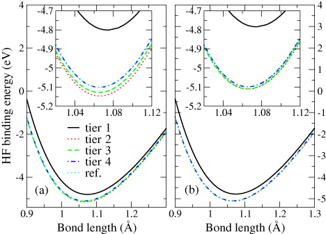
Figure 8. HF binding energy of N2 as a function of the bond length for different levels of NAO basis sets (from tier 1 to tier 4). The reference curve (denoted as 'ref') is obtained with NWChem and a Gaussian cc-pV6Z basis. (a) Results without BSSE corrections; (b) BSSE-corrected results. The insets magnify the equilibrium region.
Download figure:
Standard imageFigure 9 demonstrates the same behavior for a different test case, the binding energy of the water dimer using HF (left) and the PBE0 [7, 30] hybrid functional (right). The geometry of the water dimer has been optimized with the PBE functional and a tier 2 basis. For convenience, the binding energy is computed with reference to H2O fragments with fixed geometry as in the dimer, not to fully relaxed H2O monomers. This is sufficient for the purpose of the basis convergence test here. Detailed geometrical information for the water dimer can be found in [64]. In figure 9, the dotted line again marks the NWChem GTO cc-pV6Z reference results. Similar to the case of N2, we observe that the HF binding energy is fairly well converged at the tier 2 level, particularly after a counterpoise correction, which gives a binding energy that agrees with the NWChem reference value to within 1–2 meV. The BSSE arising from insufficient core description is reduced for the PBE0 hybrid functional, where only a fraction (1/4) of the exact exchange is included.

Figure 9. Convergence of the HF and PBE0 binding energies of the water dimer (at the PBE geometry, pictured in the inset) as a function of NAO basis size (tiers 1, 2, 3 for the first three points and tier 3 for H plus tier 4 for C for the last point). Results both with and without counterpoise BSSE correction are shown. The dotted line marks the NWChem/cc-pV6Z value.
Download figure:
Standard imageIn practice, HF calculations at the tier 2 level of our NAO basis sets yield accurate results for light elements. Counterpoise corrections help us to cancel residual total-energy errors arising from a non-HF minimal basis. However, even without such a correction, the convergence level is already pretty satisfying (the deviation between the black and the red curve in figure 9 is well below 10 meV for tier 2 or higher).
5.1.2. Heavy elements
For heavier elements (Z > 18), the impact of non-HF core basis functions on HF total energies is larger. However, the error again largely cancels in energy differences, as will be shown below. In order to avoid any secondary effects from different scalar-relativistic approximations to the kinetic energy operator, in figure 10 (upper panels) we first compare the convergence of non-relativistic (NREL) HF total energies with NAO basis size for the coinage metal dimers Cu2, Ag2 and Au2 at a fixed binding distance, d = 2.5 Å. (The experimental binding distances are 2.22 Å [163], 2.53 Å [164, 165] and 2.47 Å [163], respectively.) Again, we find that KLI-derived minimal basis sets are noticeably better converged (lower total energies) than LDA-derived minimal basis sets. In contrast to N2, however, absolute convergence of the total energy is here achieved in none of these cases, and the discrepancy increases from Cu (nuclear charge Z = 29) to Au (Z = 79).

Figure 10. Convergence with basis size of the non-relativistic (NREL) HF total energies (upper panels), non-relativistic binding energies (middle panels) and scalar-relativistic (scaled ZORA [64, 158]) binding energies (bottom panels) of Cu2 (left), Ag2 (middle) and Au2 (right), at a fixed bond length, d = 2.5 Å. Similar to figure 7, results are shown for two sets of minimal basis generated using LDA and KLI atomic solvers. For clarity the NREL total energies are offset by −89197.12, −282872.42 and −972283.08 eV, respectively, for Cu2, Ag2, Au2, which correspond to the actual values of the last data points with KLI minimal basis. All binding energies are BSSE corrected. The dashed horizontal lines in the bottom panels mark the NWChem reference values using aug-cc-pV5Z-PP basis with ECP.
Download figure:
Standard imageFor comparison, the middle and lower panels of figure 10 show non-relativistic and scalar-relativistic binding energies for all three dimers. The scalar-relativistic treatment employed is the scaled ZORA due to Baerends and co-workers [158] (for details of our own implementation, see [64]). In all three cases, the binding energies are converged to a scale of ∼0.02 eV, at least two orders of magnitude better than total energies. In other words, any residual convergence errors due to the choice of minimal basis (LDA or KLI instead of HF) cancel out almost exactly. To compare our prescription to that generally used in the quantum chemistry community where effective core potentials (ECP) are used to describe the core electrons and the relativistic effect, we also marked in figure 10 the reference values computed using NWChem and the aug-cc-pV5Z-PP basis [166, 167]. The agreement between our all-electron approach and the GTO-ECP one is pretty decent for Ag2 and Au2, whereas a larger discrepancy of ∼0.03 eV is observed for Cu2. For this particular case, we suspect that the remaining disagreement is an issue with respect to the atomic reference energy for the Cu atom between both codes. More work will be done to fully unravel the point.
5.2. MP2, RPA and GW calculations
In the implementation described here, the MP2, RPA and GW methods require the explicit inclusion of unoccupied single-particle states. As a consequence, noticeably larger basis sets are needed to obtain converged results in these calculations [38, 86, 90, 168–174]. Much experience has been gained in the quantum chemistry community to construct Gaussian basis sets for correlated calculations [157, 175], but for NAOs this is not the case. In this section, we show how our standard NAO basis sets perform for MP2, RPA and GW calculations, for both light and heavy elements. For clarity, we separate the discussions for the convergence of binding energies (in the case of MP2 and RPA) and quasiparticle excitations (in the case of GW and MP2 self-energy calculations). In contrast to the cases of HF and hybrid density functionals, BSSE corrections for RPA and/or MP2 are essential to obtain reliable binding energies. This results directly from the larger basis sets required to converge the MP2 or RPA total energy [38, 86, 90, 168–171], yielding larger BSSE for finite basis set size. With our standard NAO basis sets, the actual BSSEs in MP2 and RPA (based on the HF reference, denoted as RPA@HF in the following) calculations are plotted in figure 11 for the example of N2. The size of BSSEs in these cases is huge and does not diminish even for the pretty large tier 4 basis. It is thus mandatory to correct these errors in MP2 and RPA calculations to get reliable binding energies. As one topic of primary interest in this work is the applicability of standard NAO basis sets for MP2 and RPA, all binding energies presented are therefore counterpoise-corrected. In all HF reference calculations in this session, the KLI minimal basis is used. For RPA, GW and MP2 self-energy calculations, we use 40 imaginary frequency points on a modified Gauss–Legendre grid (appendix C), which ensures a high accuracy for the systems studied here.
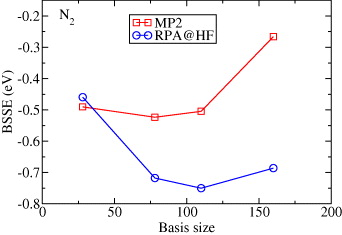
Figure 11. BSSEs in MP2 and RPA@HF binding-energy calculations for N2 (d = 1.1 Å) as a function of the NAO basis set size. The four points correspond to NAO tier 1 to tier 4 basis sets, respectively.
Download figure:
Standard image5.2.1. Binding energies
As illustrating examples for light elements, in figure 12 the BSSE-corrected MP2 and RPA binding energies for N2 and the water dimer are shown as a function of the NAO basis set size. The dotted line marks reference results computed with FHI-aims and the Dunning aug-cc-pV6Z basis. In the case of MP2, the FHI-aims aug-cc-pV6Z values agree with those of NWChem to within 0.1 meV. Unfortunately, a similar independent reference is not available for RPA, but excellent agreement is also seen with smaller basis sets, for which reference RPA data are available for N2 [38]. Upon increasing the basis size, the biggest improvement occurs when going from tier 1 to tier 2, with further, smaller improvements from tier 2 to tier 4. For the strongly bonded N2 the MP2 binding energy at tier 4 level deviates from the aug-cc-pV6Z result by ∼120 meV or ∼1% of the total binding energy. For the hydrogen-bonded water dimer, the corresponding values are ∼3 meV and ∼1.5%, respectively. The convergence quality of RPA results with respect to the NAO basis set size is similar.

Figure 12. Convergence of BSSE-corrected MP2 and RPA@HF binding energies for N2 (d = 1.1 Å) and the water dimer (PBE geometry) as a function of the NAO basis set size. The first four points correspond to NAO tier 1 to tier 4 basis sets and the last point corresponds to the composite 'tier 4 + a5Z-d' basis. The dotted horizontal line marks the aug-cc-pV6Z results.
Download figure:
Standard imageGoing beyond our FHI-aims standard NAO basis sets, further improvements arise by adding (ad hoc, as a test only) the diffuse functions from a GTO aug-cc-pV5Z basis set, denoted as 'a5Z-d' in the following. The results computed using this composite 'tier 4 + a5Z-d' basis are shown by the last point in figure 12. The deviation between the tier 4 and aug-cc-pV6Z results is then reduced by more than a factor of two. For the water dimer, for example, 'tier 4 + a5Z-d' gives −220.9 and −206.5 meV for the MP2 and RPA@HF binding energies, comparable to the quality of the cc-pV6Z basis that yields −221.1 and −206.9 meV, respectively. Both then agree with the aug-cc-pV6Z results (−222.3 meV for MP2 and −208.9 meV for RPA@HF) to within ∼2 meV.
In this context, it is interesting to check if the cut-off radii of our NAO functions have any influence on the convergence behavior demonstrated above. As described in [64], the NAO basis functions are strictly localized in a finite spatial area around the nuclei, and the extent of this area is controlled by a confining potential. For the default settings used in the above calculations, this potential sets in at a distance of 4 Å from the nucleus and reaches infinity at 6 Å. The question is: what would happen if we reduced or increased the onset radii of this confining potential? The answer to this question is illustrated in figure 13 where the basis convergence behaviors for N2 and the water dimer are shown for three different onset distances of the confining potential. From figure 13 one can see that increasing the onset radius of the confining potential (i.e. enlarging the extent of the NAO basis functions) from the default value (4 Å) has little effect on the convergence behavior for N2 or (H2O)2. Upon reducing it, noticeable changes in the results only occur for tier 1 or tier 2 in certain cases, but the overall effect is very small and does not change the general convergence behavior described above. This finding holds in general for covalent and hydrogen bonds. In practice, the onset radius may always be invoked as an explicit convergence parameter—for instance, much more weakly bonded (dispersion bonded) systems benefit from slightly larger radii (5 –6 Å) in our experience. Further details of this can be found in [176].

Figure 13. Convergence of the BSSE-corrected MP2 and RPA@HF binding energies for N2 (d = 1.1 Å) and the water dimer (PBE geometry) as a function of the NAO basis set size. The four points correspond to the tier 1 to tier 4 basis. The NAO basis functions are generated for three onset radii (3 , 4 and 6 Å) for the confining potential. The dotted horizontal line marks the aug-cc-pV6Z results.
Download figure:
Standard imageWe next illustrate the NAO basis convergence for heavy elements, using Au2 as an example. In figure 14 the MP2 binding energy for the Au2 dimer as a function of the bond length is plotted for different NAO basis sets. Relativity is again treated at the scaled ZORA level [64, 158]. The binding curves shown here demonstrate that the same qualitative convergence behavior as for our light-element test cases carries over. In essence, significant improvements are gained from tier 1 to tier 2, and basis sets between tiers 2 and 4 yield essentially converged results. For comparison, we show a completely independent (NWChem calculations) curve with Gaussian 'aug-cc-pV5Z-PP' basis sets [166, 167]. The resulting binding energy curve yields rather close agreement with our all-electron, NAO basis set results.

Figure 14. Convergence of the BSSE-corrected MP2 binding energy curve for Au2 with respect to the optimized NAO basis set size (tiers 1–4). Results from an independent, Gaussian-type calculation (aug-cc-pV5Z-PP basis set with ECP, NWChem code) are included for comparison.
Download figure:
Standard image5.2.2. Quasiparticle energies
After the discussion of binding energies, we next examine how the GW and MP2 quasiparticle energy levels converge with our NAO basis sets. The G0W0@HF and MP2 quasiparticle HOMO levels for N2 and the water dimer are plotted in figure 15 as a function of basis set size. MP2 is denoted here as 'MP2-QP' to emphasize that the MP2 self-energy (32) is used, rather than an MP2 total-energy difference. We again take the results of an 'aug-cc-pV6Z' GTO calculation as a reference. The first four data points in each sub-plot correspond to the NAO basis sets. The last point represents the composite 'tier 4 + a5Z-d' basis as described above. Once again, the biggest improvement occurs when going from tier 1 to tier 2. However, the deviation of the HOMO levels from the reference values at tier 2 level is still considerable, ∼0.2–0.3 eV for G0W0 and ∼0.1–0.2 eV for MP2-QP. These errors are brought down to ∼0.1 eV for G0W0 and ∼0.06 eV for MP2-QP by going to a pure tier 4 NAO basis set. The remaining error is then further reduced by a factor of two by including the diffuse 'a5Z-d' part of a 5Z GTO basis set. Accounting for the possible underconvergence of the aug-cc-pV6Z itself (compared to the CBS limit), we expect an overall ∼0.1 eV under-convergence of the composite 'tier 4 + a5Z-d' results given here. This is still an acceptable accuracy, considering the generally known challenge of converging the correlation contribution involving virtual states using local orbital basis functions [38, 86, 90, 168–171]. Therefore 'tier 4 + a5Z-d' basis sets were used in the benchmark calculations presented in section 6.

Figure 15. Convergence of the quasiparticle highest occupied molecular orbital (HOMO) level of N2 and the water dimer obtained with the MP2-QP and G0W0@HF self-energies versus basis size. The last data point corresponds to the composite 'tier 4 + a5Z-d' basis. The aug-cc-pV6Z result is marked by the dotted horizontal line.
Download figure:
Standard image5.2.3. G0W0 calculations for the benzene molecule
G0W0 calculations for molecules have been reported in a number of publications in recent years using various numerical frameworks and computer code packages. In particular in the solid-state community, calculations have been based on plane wave methods together with the supercell approach and pseudopotential approximations. Their advantage is a systematically convergible basis set (plane waves), especially for the unoccupied spectrum. However, the two approximations mentioned above (pseudopotential and supercell) can be drastic [177–183]. In particular, the Coulomb operator in vacuum is not screened in a standard plane wave approach. As a result, different images of the system interact with one another across supercell boundaries [179–183]. In addition, the slow convergence of G0W0 results with the plane-wave cutoff of the unoccupied spectrum is notorious [174, 184, 185].
Table 3 reports the literature G0W0 results for the benzene molecule [128, 153, 185–188], a particularly often studied case, in comparison to our own results. We focus on G0W0@LDA and G0W0@HF for the HOMO and LUMO levels. Based on these results, it is clear that there is a significant degree of scatter, even between results that are ostensibly converged using the same fundamental approximations. Our own results for NAO 'tier 3', 'tier 4' and 'tier 4 + a5Z-d' basis sets suggest internal convergence at the 'tier 4' level: −9.06 eV for the HOMO and 0.94 eV for the LUMO in G0W0@LDA, compared to −9.64 eV and 1.51 eV in G0W0@HF. The LUMO values are unbound and can be interpreted as experimental resonance energies (here taken from the tabulated negative vertical electron affinity). In either case (HOMO or LUMO, G0W0@LDA or G0W0@HF) the results are not far from the experimental values.
Table 3. G0W0 HOMO and lowest unoccupied molecular orbital (LUMO) values for the benzene (C6H6) molecule obtained by FHI-aims and several other numerical approaches as reported in the literature. 'A.E.' and 'P.P.' in the second column refer to 'all electron' and 'pseudopotential', respectively.
| G0W0-type | P.P./A.E. | Basis type | HOMO (eV) | LUMO (eV) |
|---|---|---|---|---|
| G0W0@LDA | A.E. | NAO 'tier 3'a | −8.99 | 1.06 |
| NAO 'tier 4'a | −9.06 | 0.96 | ||
| NAO 'tier 4+a5Z-d'a | −9.05 | 0.94 | ||
| P.P. | Plane waves+NAOsb | −9.03 | 1.54 | |
| Plane waves + extrapolc | −9.10 | – | ||
| Plane waves + Lancosd | −9.40 | – | ||
| NAO 'TZDP'e | −8.78 | 1.24 | ||
| Real-space gridf | −9.88 | 0.47 | ||
| G0W0@HF | A.E. | NAO 'tier 4'a | −9.64 | 1.51 |
| Gaussian 'cc-pVTZ'g | −9.28 | – | ||
| Experiments | −9.24h | 1.12i |
aThis work. bSamsonidze et al [185]: Plane wave basis augmented with siesta-type localized atomic orbitals. cUmari et al [128]: Plane wave basis extrapolated to infinite energy cutoff. dUmari et al [187]: Plane wave basis plus Lanczos trick to remove the empty states. eFoerster et al [153] fTiago and Chelikowsky [186]. gKe [188]. hNemeth et al [189]: (negative) IE. The vertical IE only differs from this value by 0.01 eV according to the NIST database (http://cccbdb.nist.gov). iBurrow et al [190]: (negative) vertical electron affinity (IE).
The same cannot be said for the comparison between the different numerical implementations. For instance, the HOMO values in G0W0@LDA range from −8.78 eV (small numeric basis set and pseudopotentials) to −9.88 eV on a real-space grid. Even within the plane wave-based approaches, the values range from −9.03 eV to −9.40 eV. Similar discrepancies arise for G0W0@HF and for the LUMO values. Within the scatter evidenced by table 3, we believe that our own results possess some merit, as the system (i) is isolated (no supercell), (ii) is treated as fully all-electron and (iii) any residual convergence issue of the unoccupied spectrum should be exposed by the diffuse Gaussian basis functions ('a5Z-d').
6. Basis set converged benchmark data for the G2 and S22 molecular test sets
Our final section utilizes the preceding methodologies and techniques to provide accurate all-electron results for molecular test sets close to basis set convergence. We cover vertical IEs and binding energies at different levels of theory, for well-defined, published molecular geometries.
6.1. Vertical IEs from HF, MP2 and G0W0 methods
The G0W0 method has been used to calculate the single-particle properties for various small- and medium-size molecules with considerable success [128, 153, 186, 188, 191–200]. The dependence of G0W0 on the starting point has also been looked at in the past [60, 61, 195, 200]. Here, using a selected collection of atoms and molecules from the G2 ion test set for IEs [79], we aim to establish the overall performance of G0W0 for computing IEs close to the basis set limit, and systematically examine its dependence on the starting point. The selection of molecules is based on the availability of experimental geometries and experimental vertical IEs. With vertical IEs we denote IEs at fixed geomerty, i.e. no structural relaxation after excitation. This quantity is directly comparable to the GW and MP2-QP quasiparticle energies. We will also assess the MP2-QP approach for determining IEs since this method was used in quantum chemistry in past decades, but direct comparisons in the literature are scarce [44]. Finally, results for IEs determined by MP2 total energy differences (denoted here simply as 'MP2' in contrast to 'MP2-QP') between the neutral atoms/molecules and the corresponding positively charged ions are also presented. We note that IEs given by MP2-QP essentially correspond to the MP2 total energy difference if the HF orbitals of the neutral systems were used in the ionic calculation (for a discussion, see, e.g., [44]). All calculations were performed at the experimental geometries. As mentioned above, the composite 'tier 4 + a5Z-d' basis set is used for most of the elements except for a few cases (e.g. rare gas atoms) where the tier 4 NAO basis is not available. In these cases, the full aug-cc-pV5Z functions are added to the NAO tier 2 basis. On average we expect the chosen basis setup to guarantee a convergence of the HOMO quasiparticle levels to ∼0.1 eV or better for the calculations presented in the following.
In figure 16, we present histograms of the error distributions given by HF, MP2-QP, G0W0@HF and G0W0@PBE0 for this database. The actual IE values are presented in appendix B. Compared to HF, one can see that the deviations from the experimental values are much smaller in G0W0 and MP2-QP. On average HF tends to overestimate IEs. This trend is corrected by MP2 and G0W0. Using the same HF reference, the magnitude of the correction is smaller in G0W0 than in MP2-QP, due to the renormalization effect coming from the screened Coulomb interaction in the GW self-energy. Concerning the starting-point dependence of the G0W0 method, G0W0 based on HF gives too large IEs on average, whereas G0W0 based on PBE does the opposite. Consequently, G0W0 based on the hybrid density functional PBE0 appears to be the best compromise, although a slight underestimation of the IEs is still visible. Furthermore, comparing MP2-QP with MP2 shows that the two approaches yield very similar results, implying that for the light elements reported here orbital relaxation effects are not significant4. Table 4 summarizes the error statistics. For the subset of atoms and molecules, MP2-QP gives the smallest mean error (ME) and G0W0@PBE0 the smallest mean absolute error (MAE).

Figure 16. Histograms of the error distribution for IEs for a set of 50 atoms and molecules calculated with HF, G0W0@HF, G0W0@PBE, G0W0@PBE0, MP2-QP and MP2.
Download figure:
Standard imageTable 4. ME, MAE and mean absolute percentage error (MAPE) for the IEs in the G2-I subset computed with HF, MP2-QP, MP2 and G0W0 based on HF, PBE and PBE0.
| ME (eV) | MAE (eV) | MAPE(%) | |
|---|---|---|---|
| HF | 0.48 | 0.70 | 5.8 |
| MP2-QP | −0.04 | 0.40 | 3.3 |
| MP2 | 0.15 | 0.31 | 2.7 |
| G0W0@HF | 0.41 | 0.52 | 4.6 |
| G0W0@PBE | −0.49 | 0.53 | 4.6 |
| G0W0@PBE0 | −0.15 | 0.25 | 2.2 |
6.2. Benchmark MP2 and RPA results for the G2-I atomization energies
The 55 atomization energies from the original G2-I set (table 3 of [201]) serve as a good benchmark database for ground-state total-energy methods for covalently bonded systems. In table 5, we present our MP2 and RPA atomization energies for the G2-I set as computed using FHI-aims and the 'tier 4 + a5Z-d' basis set. The geometries used in the calculations are those determined by Curtiss et al [201], i.e. all-electron MP2 optimization with a Gaussian 6-31G* basis set. The reference data, taken from [202], are derived from experiment and corrected for zero-point vibrations.
Table 5. G2-I atomization energies computed with MP2, RPA@HF and RPA@PBE. All numbers have been calculated with FHI-aims and 'tier 4 + a5Z-d' basis sets. The experimental reference results are taken from [202].
| Molecule | MP2 | RPA@HF | RPA@PBE | Expt |
|---|---|---|---|---|
| BeH | 54.3 | 55.6 | 49.9 | 49.8 |
| C2H2 | 412.9 | 374.1 | 377.3 | 403.4 |
| C2H4 | 564.3 | 527.4 | 533.1 | 562.4 |
| C2H6 | 709.9 | 671.4 | 678.7 | 712.7 |
| CH | 80.0 | 75.7 | 80.5 | 83.9 |
| CH2(1A1) | 176.6 | 168.1 | 173.3 | 180.9 |
| CH2(3B3) | 189.3 | 181.0 | 178.2 | 190.2 |
| CH3 | 304.6 | 290.5 | 292.4 | 307.9 |
| CH3Cl | 397.1 | 370.1 | 368.0 | 394.5 |
| CH3OH | 515.7 | 475.8 | 486.2 | 512.8 |
| CH3SH | 466.5 | 432.2 | 446.2 | 473.7 |
| CH4 | 416.1 | 395.8 | 402.4 | 420.1 |
| CN | 165.8 | 138.6 | 170.1 | 181.0 |
| CO | 270.8 | 234.7 | 241.9 | 259.3 |
| CO2 | 412.1 | 350.9 | 358.9 | 389.1 |
| CS | 178.3 | 147.9 | 154.7 | 171.2 |
| Cl2 | 64.5 | 50.1 | 45.8 | 58.0 |
| ClF | 67.2 | 47.2 | 47.4 | 61.5 |
| ClO | 61.3 | 43.3 | 56.7 | 64.6 |
| F2 | 42.6 | 16.0 | 28.4 | 38.2 |
| H2CO | 381.4 | 343.1 | 351.6 | 373.7 |
| H2O | 235.6 | 212.1 | 220.8 | 232.7 |
| H2O2 | 274.4 | 231.7 | 252.2 | 268.7 |
| H2S | 179.8 | 167.6 | 170.0 | 182.5 |
| HCN | 322.3 | 281.4 | 295.6 | 311.7 |
| HCO | 287.2 | 251.3 | 260.3 | 278.5 |
| HCl | 107.0 | 98.0 | 92.7 | 106.4 |
| HF | 145.2 | 129.4 | 130.3 | 141.1 |
| HOCl | 168.5 | 138.3 | 148.8 | 164.6 |
| Li2 | 18.2 | 13.5 | 18.3 | 24.4 |
| LiF | 145.2 | 127.3 | 125.4 | 138.9 |
| LiH | 53.2 | 50.5 | 54.1 | 58.0 |
| N2 | 238.0 | 196.3 | 219.9 | 228.5 |
| N2H4 | 436.4 | 393.8 | 421.5 | 438.6 |
| NH | 79.2 | 74.1 | 81.3 | 83.6 |
| NH2 | 178.0 | 164.6 | 177.3 | 182.0 |
| NH3 | 295.3 | 271.9 | 288.0 | 298.0 |
| NO | 155.2 | 120.2 | 145.5 | 152.8 |
| Na2 | 13.1 | 8.7 | 14.2 | 17.0 |
| NaCl | 101.3 | 91.5 | 88.7 | 97.8 |
| O2 | 129.8 | 95.4 | 110.8 | 120.3 |
| OH | 106.6 | 96.5 | 102.0 | 106.7 |
| P2 | 118.1 | 92.2 | 112.1 | 117.2 |
| PH2 | 145.7 | 140.7 | 148.2 | 153.1 |
| PH3 | 231.6 | 221.7 | 231.9 | 243.6 |
| S2 | 100.6 | 79.1 | 89.9 | 101.7 |
| SO | 132.7 | 104.6 | 110.9 | 125.0 |
| SO2 | 273.8 | 206.6 | 232.9 | 258.4 |
| Si2 | 73.7 | 64.6 | 67.7 | 74.7 |
| Si2H6 | 518.4 | 500.9 | 506.6 | 530.6 |
| (SiH21A1) | 146.4 | 140.8 | 146.5 | 151.7 |
| (SiH23B1) | 127.0 | 124.0 | 124.7 | 130.9 |
| SiH3 | 219.2 | 213.4 | 217.1 | 227.0 |
| SiH4 | 314.5 | 306.2 | 310.4 | 322.0 |
| SiO | 204.3 | 170.0 | 179.0 | 191.7 |
| ME | 1.0 | −21.5 | −13.3 | |
| MAE | 5.9 | 21.7 | 13.3 | |
| MAPE | 4.3% | 13.4% | 7.6% |
Our MP2 and RPA results are in good agreement with those reported by Feller and Peterson [203] and Paier et al [90], respectively, both obtained with GTO basis sets and extrapolated to the CBS limit. Table 5 demonstrates that MP2 performs best for these small covalently bonded molecules. The RPA approach, on the other hand, which has a broader applicability (e.g. bond breaking and/or metals where MP2 fails), exhibits significant underbinding. For RPA we also observe that KS-PBE provides a much better reference than HF. Recently, computational approaches to overcome the underbinding behavior of the standard RPA scheme have been proposed. These comprise contributions from single excitations [40] and second-order screened exchange [90, 110].
6.3. Benchmark MP2 and RPA binding energies for the S22 molecular set
The S22 molecular set proposed by Jurečka et al [80] has become a standard benchmark database for testing the accuracy of existing and newly developed methods for the description of weak interactions. S22 represents an 'unbiased' set in the sense that it contains molecules of different bonding nature (7 hydrogen bonded, 8 dispersion bonded and 7 with a mixed bonding character) and of different size (ranging from small ones like the water dimer to relatively large ones like the adenine–thymine dimer containing 30 atoms). The MP2 and CCSD(T) interaction energies for this set of molecules were already computed by Jurečka et al and extrapolated to the Gaussian complete basis set (CBS) limit. A more consistent and accurate extrapolation for the CCSD(T) values was recently carried out by Takatani et al [204], which we therefore adopt as the reference here. RPA-type calculations for S22 have recently been reported [40, 98, 205]. The agreement between the data from different groups is not perfect, and the basis incompleteness could be an issue. Of our own RPA numbers, only the MAEs and MAPEs have been reported previously [40]. Now in table 6 the actual MP2, RPA@HF and RPA@PBE binding energies for these molecules as computed using FHI-aims and the composite 'tier 4 + a5Z-d' basis set are presented. With our basis setup, the MP2 binding energies are underestimated by ∼4.5 meV (2% on a relative scale) compared to the MP2/CBS results reported in [80]. We expect a similar convergence of the RPA numbers based on our basis set convergence tests shown in previous sections. Compared to the CCSD(T) reference data, RPA@PBE, which nowadays dominates RPA-type production calculations, systematically underestimates all of the three weak bonding categories and gives an MAE of 39 meV and an MAPE of 16%. If instead HF is used as a starting point (i.e. as for MP2), the description of hydrogen bonding improves, while the description of dispersion bonding worsens. The overall MAE for RPA@HF is 51 meV and the MAPE 25%. We are thus faced with the conundrum that RPA can describe the weak interactions that are beyond the reach of LDA, GGA and hybrid functionals, but the accuracy of the two standard RPA schemes is not spectacular. We have analyzed the origin of this underbinding behavior in [40] and proposed a simple solution to overcome this problem.
Table 6. Binding energies (in meV) of the S22 molecular set [80] calculated with MP2, RPA@HF and CCSD(T). MP2 and RPA results have been obtained with FHI-aims and 'tier 4 + a5Z-d' basis sets. The reference CCSD(T) results are from [204].
| Molecules | MP2 | RPA@HF | RPA@PBE | CCSD(T) | |
|---|---|---|---|---|---|
| 1 | NH3 dimer | 136 | 116 | 112 | 137 |
| 2 | H2O dimer | 214 | 201 | 182 | 218 |
| 3 | Formic acid dimer | 799 | 790 | 744 | 816 |
| 4 | Formamide dimer | 681 | 662 | 645 | 700 |
| 5 | Uracil dimer | 881 | 846 | 816 | 898 |
| 6 | 2-pyridoxine.2-pyridoxine | 749 | 666 | 678 | 738 |
| 7 | Adenine.thymine | 714 | 639 | 658 | 727 |
| 8 | CH4 dimer | 21 | 11 | 17 | 23 |
| 9 | C2H4 dimer | 67 | 37 | 49 | 65 |
| 10 | Benzene CH4 | 78 | 35 | 49 | 63 |
| 11 | Benzene dimer | 211 | 40 | 82 | 114 |
| (slip parallel) | |||||
| 12 | Pyrazine dimer | 296 | 110 | 144 | 182 |
| 13 | Uracil dimer | 482 | 310 | 379 | 423 |
| 14 | Indole.benzene | 345 | 86 | 148 | 199 |
| 15 | Adenine.thymine (stack) | 641 | 388 | 422 | 506 |
| 16 | Ethene.ethine | 72 | 57 | 54 | 65 |
| 17 | Benzene.H2O | 153 | 119 | 123 | 143 |
| 18 | Benzene.NH3 | 114 | 74 | 85 | 101 |
| 19 | Benzene.HCN | 223 | 178 | 170 | 197 |
| 20 | Benzene dimer (T-shape) | 156 | 75 | 96 | 118 |
| 21 | Indole.benzene (T-shape) | 200 | 182 | 215 | 244 |
| 22 | Phenol dimer | 334 | 250 | 266 | 308 |
| ME | 26 | 51 | 39 | ||
| MAE | 37 | 51 | 39 | ||
| MAPE | 19% | 25% | 16% |
7. Conclusions and outlook
To summarize, we have presented an RI framework for the two-electron Coulomb operator that allows efficient, accurate electronic structure computations with HF, hybrid functional, MP2, RPA and GW methods based on the flexible basis function form of NAOs. We have shown that NAO basis sets as implemented in FHI-aims are a competitive choice for approaches involving exact-exchange and/or non-local correlation terms, with rather compact basis sets sufficing for essentially converged results. Our simple 'on-the-fly' scheme to construct the ABFs using the Gram–Schmidt orthonormalization of the 'on-site' products of single-electron atomic orbitals gives a natural, accurate representation of the two-electron Coulomb operator for practical calculations. Taken together, our framework paves the way for an extended usage of NAOs in more advanced computational approaches that go beyond LDA and GGAs. Specifically, we have applied the G0W0 and MP2 quasiparticle approaches to compute the vertical IEs of a set of small molecules, and the RPA method to compute the G2-I atomization energies and the interaction energies for the S22 molecular set. We believe that the well-converged numbers reported in this work may serve as benchmarks for future studies. Beyond the specific examples given here, our RI framework as a whole has already proven to be stable and mature in a number of scientific applications [40, 41, 96, 176, 206–208].
Based on the results above, NAOs emerge as a promising route towards more compact basis sets for correlated methods. Among our ongoing developments is the attempt to design more optimized NAO basis sets for MP2, RPA and GW calculations. Another active line of development is to improve the scaling behavior of the computational cost with system size, exploiting the locality of the NAO basis functions [147]. Last but not least, we are working on the extension of the present scheme to periodic systems. All this combined, we expect NAO-based implementations of methodologies that go beyond LDA and GGAs to become competitive alternatives to the traditional implementations that are based on GTO or plane-wave basis sets, in particular towards the limit of very large systems: the benefit of compact basis set size at a given accuracy level should help tackle problem sizes that, otherwise, could not be done.
Acknowledgments
We acknowledge fruitful discussions with and encouragement by an extensive group of friends, coworkers and colleagues over the many years that our approach has been in productive use. This work was in part funded by the EU's Sixth Framework Programme through the NANOQUANTA (NMP4-CT-2004-500198) network of excellence and the EU's Seventh Framework Programme through the European Theoretical Spectroscopy Facility e-Infrastructure grant (no. 211956).
Appendix A.: Matrix elements for numeric atom-centered orbitals
A.1. Coulomb potential of a numerical radial function
To reduce the (formally) 6D Coulomb integrations to 3D ones, we first solve Poisson's equation for each Pμ(r') (classical electrostatics). We define Qμ(r) as

Using the Laplace expansion of the Coulomb potential v(r − r') = 1/|r-r'|,

where r< = min(r,r') and r> = max(r,r'), the integration of the angular part in (A.1) can be done analytically, yielding

The radial part αalκ(r) is given by a simple 1D (numerical) integration [64, 65, 209]

Thus, the three-center and two-center Coulomb integrals (37) and (45) reduce to the 3D integrals in (66) and (67).
A.2. Grid-based three-center and two-center integrals
The three-center and two-center integrals in this work are computed by grid-based integrations using overlapping, atom-centered spherical grids and the same technology that is used in many quantum-chemical applications for the XC matrix in the DFT [65, 154]. The integration grid points r = r(a,s,t) are uniquely specified by the atomic center a, the radial shell number s and the angular point t. w(s,t) is the corresponding integration weight. Details of our own implementation (FHI-aims) are given in [64, 155]. Since these are true three-center integrals, we restrict the integration domain for a particular integral element to the grids associated with the atoms on which the basis functions in question are centered. For instance, denoting the respective atoms by a1, a2, a3, the three-center integrals in (66) can then be discretized as

where p3(a,r) is a three-center partition function that satisfies

everywhere in the overlapping region of the three functions, and is zero otherwise. The underlying numerical grids can, in principle, be increased up to arbitrary accuracy if needed. The two-center integrals (67) can be performed in a similar fashion using overlapping grids, or with the spherical Bessel transform techniques explained below.
A.3. Two-center integration in Fourier space
As mentioned in section 4.3, two-center integrals of numeric atom-centered basis functions like Vμν in (37) and Sμν in (41) can be efficiently calculated in Fourier space as described by Talman [132, 210]. This and the following (appendix A.4) subsections give the details of our implementation. We first describe the general procedure here, and the central ingredient of our implementation, the logarithmic spherical Bessel transform (logarithmic SBT (logSBT)), will be presented in the next subsection.
As is well known, the overlap of two functions f(r) and g(r) can be expressed in Fourier space as

The Fourier transform in (A.6) of an atomic function has the same angular momentum in real and Fourier space for symmetry reasons


The radial part is given by the SBT of f(r)


If f(r) is tabulated on a logarithmic grid, its SBT can be calculated efficiently on an equivalent logarithmic grid using the fast logSBT algorithm [211–213] as described in the next section.
The 3D integral (A.6) can be separated by expanding the plane wave eik·R in spherical harmonics and spherical Bessel functions

The separation yields

with a radial integral

and an angular integral

The triple-Y integrals

in (A.12) can be calculated efficiently using recursion formulae [210]. They are non-zero only for L = |l − l'|,|l − l'| + 2,...,(l + l'). If two atom-centered functions do not overlap, the overlap integrals IL(R) of course vanish.
For a given distance R, the radial integrals IL(R) in (A.11) can be calculated directly using the trapezoidal rule on the logarithmic grid when jL(kR) is evaluated in logarithmic Fourier space as described in the next section. If integrals of the same atom-centered functions for many differing distances are needed, one can compute these more efficiently by interpreting (A.11) as an SBT of . By applying logSBT, and interpolating for all needed distances R, one can obtain all the integrals at tight-binding cost, meaning that an efficient recursion formula (together with spline evaluations) can be used instead of evaluating each integral numerically.

Coulomb interactions of atomic functions can be calculated with comparable ease where the integrand in (A.11) is multiplied with the Coulomb kernel 4π/k2

The Coulomb interaction generally does not vanish even if the two charge densities do not overlap. However, it has a simple multipolar behavior and explicit integration of (A.14) can thus be avoided. The function VL(R) can formally be interpreted as the far field of a charge distribution of angular momentum L whose radial part P(r) is given by its SBT . Therefore, it only depends on the multipole moment of P, which is encoded in its limiting behavior for small k. From this, it can be shown that VL(R) vanishes for all L < l + l'. For L = l + l' we get


with (2n − 1)!! = 1·3···(2n − 1) and with multipole moments

Therefore, the Coulomb interaction of non-overlapping functions depends only on the product of their multipole moments and can also be calculated at tight-binding cost.
As a side remark, we emphasize that two ABFs do not interact via the Coulomb interaction if they do not overlap and at least one of the two multipole moments is zero. As shown by Betzinger et al in [214], all but one of the ABFs for a given atom and a given angular momentum lm can then be chosen to be multipole-free by means of a suitable unitary transformation.
A.4. Logarithmic spherical Bessel transform
This section describes our implementation of the logSBT algorithm. For a more extensive description, see Talman [213] and Hamilton [212].
The SBT as defined in (A.8) can be written as the integral over a kernel and a right-hand-side :


The choice of the power bias parameter 0 ⩽ α ⩽ 3 is crucial for the numerical accuracy and stability of this method and will be discussed further below. The basic idea of the logSBT is that in logarithmic coordinates (ρ = log r and κ = log k) the kernel reads and (A.17) turns into a convolution, which can be efficiently calculated using fast Fourier transforms (FFTs). Please note that dr/r = dρ in (A.17).

As pointed out by Hamilton [212], this procedure is exact if both and the corresponding SBT term are periodic in logarithmic space and analytic expressions for the logarithmic Fourier transform of the kernel are used. Periodicity can be achieved, e.g., by choosing α near 1.5 and using a sufficiently wide logarithmic grid. Under these circumstances, both and smoothly drop to zero on both ends, which therefore can safely be connected.


Unfortunately, the scaling factor k−α turns out to be quite problematic. By the design of the algorithm, the absolute error of before the final scaling is typically of the order of machine precision, i. e. about 10−15. This is true even if the magnitude of the exact value is much smaller than that. After scaling, however, the absolute error can get arbitrarily large because k can be very small on a wide logarithmic grid.

Talman [213] circumvents this problem by using two separate α for small and large k and joining the two results where they differ least. The small-α (α = 0) calculation cannot be done assuming periodicity for l = 0 because does not decay to zero for ρ → − ∞. Therefore, a trapezoidal rule is used for the integration, which works well for small k where the Bessel function is smooth on a logarithmic scale. This does not break with the spirit of logSBT, because the trapezoidal rule can be formulated using FFTs, too.

In order to avoid the second transform, we take a different approach. In practice, one needs the SBT only for one kind of integral and it is sufficient to calculate to high absolute accuracy for a single given α, which can be used as power bias for the transform.

This works well for all cases but α = 0 and l = 0. Here, we cannot simply resort to the trapezoidal rule because it is invalid for high k where the Bessel function oscillates rapidly. Instead, we separate j0(eτ) into a smooth part proportional to erfc(τ/Δτ0) and a properly decaying rest. We use the first part for a trapezoidal rule and the second part for the log-periodic algorithm. Fortunately, these two schemes differ only in the way the kernel is constructed so that the two kernels can simply be added up to a 'hybrid' kernel. The actual transform is not affected and numerically not more expensive than an ordinary logSBT.
Just like Talman [213], we double the domain during the transforms for l = 0 and l = 1 in order to avoid the need for large domains for a proper decay behavior.
Appendix B.: Ionization energies of a set of atoms and molecules
In table B.1, the individual numbers for the vertical ionization potentials for 50 atoms and molecules as computed with six different computational approaches are presented. The calculations are performed with FHI-aims and 'tier + a5Z-d' basis set.
Table B.1. The vertical ionization potentials (in eV) for 50 atoms and molecules (taken from the G2 ion test set [79]) calculated with HF, MP2, MP2-QP, G0W0@HF, G0W0@PBE0 and G0W0@PBE in comparison to the experimental values taken from the NIST database (http://cccbdb.nist.gov).
| Molecule | Expt | HF | MP2 | MP2-QP | G0W0@HF | G0W0@PBE0 | G0W0@PBE |
|---|---|---|---|---|---|---|---|
| Al | 5.98 | 5.95 | 5.85 | 6.08 | 6.24 | 5.94 | 5.64 |
| Ar | 15.76 | 16.08 | 15.87 | 15.61 | 16.08 | 15.51 | 15.21 |
| B | 8.30 | 8.68 | 8.33 | 8.79 | 8.73 | 8.11 | 7.65 |
| BCl3 | 11.64 | 12.48 | 12.58 | 11.65 | 12.37 | 11.63 | 11.25 |
| BF3 | 15.96 | 18.04 | 16.19 | 15.02 | 16.77 | 15.79 | 15.21 |
| Be | 9.32 | 8.48 | 8.87 | 8.98 | 9.16 | 9.26 | 9.03 |
| C | 11.26 | 11.95 | 11.33 | 11.79 | 11.68 | 10.93 | 10.47 |
| C2H2 | 11.49 | 11.19 | 11.75 | 11.43 | 11.76 | 11.29 | 11.01 |
| C2H4 | 10.68 | 10.23 | 10.77 | 10.37 | 10.83 | 10.47 | 10.22 |
| C2H4S | 9.05 | 9.43 | 9.27 | 8.74 | 9.44 | 8.94 | 8.71 |
| C2H5OH | 10.64 | 12.05 | 11.30 | 10.08 | 11.47 | 10.63 | 10.20 |
| C6H6 | 9.25 | 9.15 | 9.88 | 9.08 | 9.63 | 9.20 | 9.00 |
| CH2CCH2 | 10.20 | 10.31 | 10.55 | 9.94 | 10.70 | 10.12 | 9.85 |
| CH2S | 9.38 | 8.24 | 9.76 | 8.04 | 8.22 | 9.27 | 9.01 |
| CH3 | 9.84 | 10.47 | 9.78 | 10.61 | 10.28 | 9.59 | 9.24 |
| CH3Cl | 11.29 | 11.87 | 11.63 | 11.20 | 11.88 | 11.31 | 11.03 |
| CH3F | 13.04 | 14.46 | 14.18 | 12.98 | 14.15 | 13.28 | 12.77 |
| CH3SH | 9.44 | 9.67 | 9.56 | 9.25 | 9.81 | 9.31 | 9.06 |
| CH4 | 13.60 | 14.85 | 14.46 | 14.18 | 14.89 | 14.27 | 13.98 |
| CHO | 9.31 | 11.13 | 9.36 | 9.92 | 10.64 | 9.61 | 9.14 |
| CO | 14.01 | 15.10 | 14.55 | 14.06 | 14.85 | 13.78 | 13.30 |
| CO2 | 13.78 | 14.83 | 14.86 | 13.29 | 14.48 | 13.68 | 13.21 |
| CS2 | 10.09 | 10.14 | 10.86 | 10.03 | 10.55 | 10.02 | 9.72 |
| Cl | 12.97 | 13.09 | 12.90 | 13.21 | 13.32 | 12.83 | 12.51 |
| Cl2 | 11.49 | 12.08 | 11.66 | 11.38 | 12.13 | 11.49 | 11.04 |
| ClF | 12.77 | 11.63 | 11.34 | 11.08 | 11.72 | 11.15 | 10.72 |
| F | 17.42 | 18.50 | 17.42 | 17.30 | 17.73 | 17.07 | 16.71 |
| FH | 16.12 | 17.70 | 16.47 | 14.93 | 16.39 | 15.83 | 15.39 |
| H | 13.61 | 13.61 | 13.61 | 13.61 | 13.61 | 13.04 | 12.52 |
| He | 24.59 | 24.98 | 24.41 | 24.58 | 24.68 | 24.01 | 23.59 |
| Li | 5.39 | 5.34 | 5.38 | 5.38 | 5.68 | 5.84 | 5.67 |
| Mg | 7.65 | 6.88 | 7.40 | 7.44 | 7.56 | 7.64 | 7.71 |
| N | 14.54 | 15.54 | 14.66 | 14.98 | 14.85 | 14.06 | 13.51 |
| N2 | 15.58 | 16.71 | 15.48 | 17.22 | 17.27 | 15.45 | 14.86 |
| NH3 | 10.82 | 11.70 | 11.06 | 10.29 | 11.36 | 10.70 | 10.32 |
| Na | 5.14 | 4.97 | 5.11 | 5.09 | 5.37 | 5.51 | 5.51 |
| NaCl | 9.80 | 9.68 | 9.42 | 9.98 | 9.59 | 9.09 | 8.79 |
| Ne | 21.56 | 23.14 | 21.63 | 20.22 | 21.76 | 21.10 | 20.54 |
| O | 13.61 | 14.20 | 13.48 | 14.64 | 13.90 | 13.37 | 13.04 |
| O2 | 12.30 | 15.22 | 11.85 | 12.57 | 13.71 | 12.33 | 11.68 |
| OCS | 11.19 | 11.47 | 11.95 | 11.16 | 11.70 | 11.16 | 10.88 |
| OH | 13.02 | 13.98 | 13.14 | 13.21 | 13.38 | 12.79 | 12.41 |
| P | 10.49 | 10.67 | 10.56 | 10.78 | 10.72 | 10.24 | 9.94 |
| P2 | 10.62 | 10.10 | 10.86 | 10.59 | 10.70 | 10.35 | 10.13 |
| PH3 | 10.59 | 10.58 | 10.58 | 10.47 | 10.90 | 10.44 | 10.22 |
| S | 10.36 | 10.33 | 10.15 | 11.04 | 10.69 | 10.31 | 10.12 |
| S2 | 9.55 | 10.38 | 9.38 | 9.74 | 10.21 | 9.39 | 9.05 |
| SH2 | 10.50 | 10.49 | 10.53 | 10.34 | 10.74 | 10.27 | 10.06 |
| Si | 8.15 | 8.20 | 8.10 | 8.33 | 8.38 | 8.01 | 7.76 |
| SiH4 | 12.30 | 13.24 | 12.81 | 12.90 | 13.33 | 12.68 | 12.29 |
Appendix C.: The modified Gauss–Legendre grid
For the integrals over the imaginary frequency axis (e.g. for the RPA correlation energy, equation (60)), we use a modified Gauss–Legendre quadrature. The Gauss–Legendre quadrature provides a way to numerically evaluate an integral on the interval [ − 1:1]

where xi and wi are the integration points and the corresponding weights, respectively. For our purposes a transformation procedure is applied to map the integration range from [ − 1:1] to [0:∞] whereby the xi and wi have to be changed accordingly. Specifically, we use the modification proposed for the evaluation of the Casimir–Polder integral (http://www.physics.udel.edu/~szalewic/SAPT/sapt2008manualse15.html):

with x0 set to 0.5. The weights for the transformed grid are then given by

This modified Gauss–Legendre scheme allows a quick convergence of the frequency integration with a relatively small number of frequency points. In our implementation, a 40-point grid gives micro-Hartree total energy accuracy for the systems investigated in this work.
Footnotes
- 3
Here and in the following, we refrain from employing any basis extrapolation strategies as often advocated in the quantum chemistry community, but rather compare to directly computed values from the largest available standard GTO basis sets. It is well known that basis set extrapolation can yield good results, especially for mid-sized GTO basis sets. However, at the meV-level convergence with very large basis sets that we are aiming for here, it is not clear what degree of residual noise should be expected from a basis set extrapolation.
- 4
For heavy elements, on the other hand, we found that the discrepancy between MP2-QP and MP2 becomes large. The discussion of this issue is beyond the scope of this paper and will be reported elsewhere.