


Abstract
Metallic gyroid metamaterials are formed by a combination of nanoplasmonic helices leading to unique and complex optical characteristics. To unravel this inherent complexity we set up an analytic tri-helical metamaterial model that reveals the underlying physical properties. This analytic tri-helical model is complete in the sense that it is only dependent on the structure's geometric and material parameters. It allows us to elucidate the characteristic transverse and longitudinal modes of the metal nano-gyroid as well as explain the surprisingly small optical chirality of gyroid metamaterials that is observed in experiments. We argue that this behaviour originates from the interconnection of multiple helices of opposing handedness.
Export citation and abstract BibTeX RIS

Content from this work may be used under the terms of the Creative Commons Attribution-NonCommercial-ShareAlike 3.0 licence. Any further distribution of this work must maintain attribution to the author(s) and the title of the work, journal citation and DOI.
1. Introduction
Metamaterials are artificial media whose electromagnetic behaviour is determined by the geometry of their sub-units. These sub-units can be specifically designed to give simultaneously a negative effective permittivity ε and permeability μ, resulting in an effective negative refractive index (n < 0), a property that cannot be observed intrinsically in any natural material. Alternatively, when chirality (handedness) is introduced in a resonant medium, then the effective response of the two circularly polarized states differ, with one of them 'experiencing' effective negative refractive index [1]. At microwave frequencies, metamaterials have been designed and manufactured to achieve extreme chirality [2], demonstrated in chiral Swiss-Rolls [1, 2], twisted layers of gammadions and crossed-wires [3, 4]. These have found numerous significant applications, such as polarizers, filters and slow waves for waveguides and antennas. During the last few years, significant efforts have been focused on moving metamaterial functionalities such as stopped light [5] from microwave to mid- and near-infrared (IR) frequencies, heralding significant technological breakthroughs in optoelectronics and photonics. However, as the constituent metamolecules should be significantly smaller than the wavelength, metamaterials that are designed for the IR regime have to have nanoscaled metamolecular sub-units. Clearly, this is not without manufacturing challenges, particularly as most common strategies rely on top-down techniques involving considerable effort [6]. Not surprisingly, there has been an increasing interest in developing bottom-up techniques such as, in particular, self assembly of nanoplasmonic gyroid structures (figure 1) [7, 8], opening a route for artificial 3D chirality at IR frequencies. First experimental results on nanoplasmonic gyroid metamaterials show very interesting behaviour [7], but at the same time pose many new questions, particularly related to the underlying physics.

Figure 1. (a) The single gyroid metamaterial and (b) the unit cell of a THM.
Download figure:
Standard imageIn this paper, we thus aim to shed light on the physics that determine the electromagnetic response of metallic single gyroid metamaterials. On the basis of a tri-helical metamaterial (THM) geometry, we develop an analytical model that describes the effective electromagnetic and chiral properties of the structure well into mid-infrared and near infrared frequencies, by considering metallic losses and the thickness of wires that previous studies have neglected [9, 10]. Our analytical model is complete, depending only on the structure's geometric and material parameters. Therefore, our analytical model derived here is a valuable tool to guide the design and fabrication of chiral structures, in particular the metal nano-gyroid operating at infrared frequencies.
2. Tri-helical metamaterial (THM)
The gyroid metamaterial shown in figure 1(a) is composed of multiple helices, connected with each other and orientated over several directions. If we now remove the connections between the helices and orient them (for simplicity) along the x, y and z axes we obtain a 3D isotropic 'THM' model system. As we discuss in this paper, the THM model bears many features of gyroid metamaterials, thus opening up a route to analytic analysis that elucidates the physical properties. In the THM each helix is created by wrapping a wire of thickness rw around a cylinder of radius R (see figure 2). The surface of the helix aligned along the z-axis is approximated by:

where u and t assume values −π ⩽ u ⩽ π and −π ⩽ t ⩽ π for one period of the helix, and p is the z-axis periodicity or pitch of the helix. The effective permittivity (  ), permeability (
  ) and chirality (
  ) tensors of the THM can then be expressed as:
Due to the 3D isotropic nature of the THM, χxxEE = χyyEE = χzzEE = χEE, χxxHH = χyyHH = χzzHH = χHH and χxyEH = χyzEH = χzxEH = ··· = χEH, reducing the effective tensors to:
where we have, for simplicity, disregarded any non-local corrections. To derive effective electromagnetic and chirality parameters, we now follow a similar approach to [2].
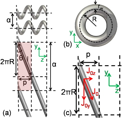
Figure 2. (a) Wire helices aligned with the z-axis (top) and unwrapped helices (bottom), where the length l of the wires per unit cell, the pitch p, the periodicity a and the angle θ the wires make with the y-axis are defined. (b) The xy-view of a helical wire, where the radius of the wire rw and the radius of the helix R are defined. (c) The current density components, shown on an unwrapped wire.
Download figure:
Standard imageLet us start by looking at wire helices aligned along the z-axis whose effective parameters along this axis are identical to χEE, χHH, χEH and χHE of the THM. These helices have a unit cell of dimensions a × a × p, as highlighted in figure 2(a). Note that (2R + 2rw) < a is imposed to ensure that the helices do not overlap. Now consider an electric field E0z also oriented along the z-axis, in order to derive the effective χEE and χEH, and a magnetic field H0z to derive the effective χHH and χHE. The H0z field induces a current density J0y on the helical wire and the E0z field a current density J0z. From figure 2(c), we see that the current densities are related as:

with θ denoting the angle between the helical wire and the y-axis, as defined in figure 2(a). Note that J0z and J0y can have negative values, which determines the handedness and current direction on the wire. Therefore, the magnetic field Hz in a unit cell, driven by J0y, is given by

where R is the radius of the helical wire as defined in figure 2(b), a is the lattice constant and l is the length of the wire per turn given by:

and is shown in figure 2(a). The term (a/l) in (5) accounts for the fact that current densities are spread over the length l of the wire, rather than the length a along the y-axis (more details in appendix). Assuming that H0z is of the form of  , then the electromotive force (emf)
  induced in a unit cell is given by:
The last term takes resistive losses in the metallic wires into account, which oppose the flowing current. The losses are expressed in terms of the surface resistivity ρ of the helical wire (measured in Ω), since the current flows on the surface of thick wires. Note that ρ also takes into account the resistivity due to field penetration into the metal (discussed in more detail in section 2.1). Additionally, the confinement of electrons in the wires gives rise to a local magnetic field around the wires that enhances the effective electron mass [11, 12]. Therefore, the electrons appear to be heavier, requiring more energy from the current flow, slowing it down and giving rise to the following self-inductance per unit cell [11, 12]:

where r0 is the radius of the wire that is not penetrated by the wave's fields and is given by r0 = rw − δ, rw is the radius of the wire and δ the skin depth. Note that the above formula for Lm holds for rw > δ. Since the magnetic field due to Lm is highly localized around the wire, it is reasonable to assume that there are no contributions from neighbouring wires (i.e. the magnetic effect due to self-inductance is negligibly small at a distance R from the wire). Therefore, the potential due to self-inductance is given by:

where we consider only the J0z component of the current density for simplicity. Since the self-inductance opposes the current flow, its magnetic effect VL needs to be subtracted from  , leading to a potential per unit cell due to magnetic effects given by:

An electric field E0z then induces the current density J0z, which drives the depolarizing fields, leading to:

where εd is the dielectric permittivity of the host medium and can take complex values. The potential difference across the z-component of the unit cell is given by:

Note that the last term reduces VE due to metallic losses. Then, assuming that there is no contribution from neighbouring unit cells and that the process is adiabatic (i.e. VE = VH), the averaged current densities (i.e. J0y and J0z) per unit cell read:

Finally, the electric permittivity (χEE), magnetic permeability (χHH) and chirality parameters (χEH, χHE) along a helix are obtained through ε−1zz = ε0Eave/Dz and μ−1zz = μ0Have/Bz respectively [13], where Dz = ε0E0z, Eave = Ez, Bz = μ0H0z and  , obtained by averaging the H-field over a line outside the helix. Therefore we obtain:


where
is the plasma frequency,

the magnetic resonance frequency and G is a constant defined as:

The loss parameters Γ and γ are given by:

Note that κ−1EH = −κ−1HE. As discussed above, although (14)–(17) express the effective parameters and chirality along a single helix, they are identical to the effective parameters along the three orthogonal axes of the isotropic THM. The inverse electromagnetic parameters are derived here, since they take a simpler form, and the non-inverse parameters can be obtained using:

where  . Although κEH and κHE express the chirality in the structure, it is often more convenient to quantify chirality in terms of the optical activity per wavelength:

The real part of ϕ is the optical rotation and measures the polarization rotation of a wave travelling through the medium. It also measures the strength of the structure's chirality. The imaginary part of ϕ shows the circular dichroism of the structure, which is a measure of the circular ellipticity of the wave in the medium.
2.1. Metallic losses at high frequencies
The analytical model accounts for metallic losses through the surface resistivity ρ, representing the dominant contribution to metallic losses, since at mid-IR and visible frequencies they have a huge impact on the electromagnetic behaviour of metallic structures. In these regimes, metals can be expressed with a Drude model:

where εm' and εm'' are the real and imaginary components of the metal's permittivity respectively, and ωp−metal and g are the plasma and collision frequencies of the metal. For specificity, we here consider silver with ε∞ = 4.028, ωp−silver = 1.39 × 10¹⁶(rad s−1) and g = 4.997 × 10¹²(1/s). Also, it is well known that the permittivity of any medium can be expressed in terms of the resistivity as [14] :

where ρm(ω) is a complex function of the frequency, with the real part representing the resistivity and the imaginary part the reactance of the medium. Note that ρm(ω) = 1/σm(ω). Then, solving (25) and (26) we obtain:

which is expressed in terms of the metal properties and is measured in terms of Ωm. The skin depth δ takes into account how far the fields can penetrate into the metal; it depends on ρm(ω) and ω as [15]:

where μm is the magnetic permeability of the metal, and for silver μm = 1. The quantity ρ in (21) and (22) is the surface resistivity of the metal, which is dominated by the penetrated metal (δ), and sometimes referred to as the internal impedance [15]:

Substituting (29) into (21) and (22), then the effect of the skin-depth and increased resistivity is accounted in our analytical model.
3. Verification of the tri-helical analytical model at mid-infrared frequencies
3.1. Scattering and effective optical parameters
We now apply our analytical model to a silver THM with parameters a = 1 μm, p = 0.5 μm, R = 0.19 μm, εd = 1 and rw = 0.06 μm. The scattering parameters plotted in figure 3(a) for a slab of thickness d = 3a = 3 μm are calculated analytically using (14)–(17) in the scattering equations of [16], and numerically using a finite integration technique2. The analytical predictions and numerical calculations show very good agreement, and as expected, the reflection coefficients for right-handed circular polarization (RCP) and left-handed circular (LCP) waves are degenerate (i.e. R = R−− = R++). A RCP or LCP wave incident on a chiral slab is reversed when reflected, and therefore the optical path of either an RCP or LCP wave is the same, resulting in identical reflection coefficients [16]. Also, as expected, the transmission coefficients for the right- (T++) and left-handed (T−−) polarizations differ, as chirality leads to two different refractive indices for the right- and left-handed polarizations.

Figure 3. Numerical (points) and analytical (lines) results are plotted together for comparison: (a) The S-parameters R = R++ = R−−, T++, T−− and the cross-coupling parameters T+− and T−+, which take small values, (b) the racemic refractive index n, (c) the refractive index for RCP wave incidence n+, (d) the refractive index for LCP wave incidence n−, (e) the chirality parameter κEH, (f) the optical activity ϕ, (g) the electric permittivity χEE and (i) the magnetic permeability χHH.
Download figure:
Standard imageThe electromagnetic parameters were retrieved from numerical scattering calculations [4] and are plotted together with (14)–(17) of the analytical model for comparison in figures 3(b)–(h), showing excellent agreement. We can immediately note that the cross-coupling transmission coefficients (T−+ and T+−) in figure 3(a) are small in the frequency range, the retrieval method was applied as required by [4]. Figures 3(b)–(h) show that the racemic refractive index  approaches zero for frequencies below the plasma frequency (ωp ∼ 40 THz) and becomes positive, since the magnetic permeability is always positive. Moreover, the refractive index for a right-handed polarized wave (n+) is always positive as expected, but the refractive index for left handed polarized waves (n−) is negative for ω < ωp. The real part of the chirality index (Re(κ)) is small and varies from negative to positive values. However, the imaginary part (Im(κ)) that dominates the optical activity, is larger. Also, the real and imaginary parts of the optical activity ϕ are maximum at ω ∼ ωp. This indicates that the chirality of the structure is strongest in this frequency range. Moreover, the small mismatch between the peaks of Re(ϕ) and Im(ϕ) shows that there are frequencies where optical rotation is dominant over circular ellipticity. Finally, as expected, the electric permittivity follows a Drude-like behaviour and the magnetic permeability a Lorentz-like resonance. The magnetic permeability is weakly resonant, and always positive when metallic losses are present, which indicates that the negative values of Re(n−) are due to the medium's chirality Im(κEH) (i.e. n± = n ± iκEH/c0) .
To further validate our analytical model for a range of different THMs and frequency regimes, we now plot in figure 4 the resonant frequencies ωp and ω0m in dependence on the structure's various geometrical parameters (rw, a, R and p) for both the analytical model (lines) and the numerical results (points). The resonance frequencies assume higher values for thicker wires and larger helix pitch p, where the model is expected to hold for p < a (i.e. p < 3 μm). Also, the analytical model shows excellent agreement for rw > δ as expected, while for rw < δ the wires are fully penetrated by the waves and a different formulation needs to be taken into account. Note that δ, also plotted in figure 4(a) with a solid black line, is a weakly dispersive quantity for this frequency regime. Finally, ω0m and ωp are reduced for larger helix radius R and needless to say, for larger lattice constants a. The excellent agreement between the analytical model and numerical results for all geometrical parameters of the THM is clear evidence that the model presented in this paper predicts with high accuracy the behaviour of metallic THMs in the presence of losses within the infrared spectrum.

Figure 4. Dependence of the THM's resonant frequencies (ω0m and ωp) on (a) the radius of the wire rw plotted together with the variation of the skin-depth δ with frequency (black solid line), (b) the lattice constant a, (c) the radius of the helices R and (d) the pitch of the helices p. Note that the model holds for rw > δ and p < a. The analytical results are plotted with lines and numerical calculations with points.
Download figure:
Standard image3.2. Band structure of THM
We now use our analytical model to calculate the dispersion diagram of the THM. Since the THM is a 3D isotropic chiral medium, the dispersion equations are given by [1]:
Equations (14)–(17) are substituted in (30) and the dispersion diagram for the THM with a = 1 μm, p = 0.5 μm, R = 0.19 μm, εd = 1 and rw = 0.06 μm is plotted in figure 5(a) with simulation results obtained using CST Microwave Studio, and show remarkable agreement. The cut-off frequency in figure 5(a) is a characteristic of wire-mesh metamaterials [11, 12, 17], which is a simplified version of THM. It has been previously discussed in the literature [1, 2] that the two degenerate transverse modes of a passive medium split in the presence of chirality. For a resonant medium (or a medium with a cut-off frequency like wire-mesh metamaterials), when the two transverse modes split in the presence of chirality, one polarization experiences effective negative refractive index for a frequency bandwidth that is dependent on the strength of the chirality, as observed in figure 5.
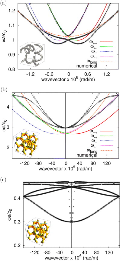
Figure 5. Band structures for (a) PEC THM of dimensions a = 1 μm, p = 0.5 μm, R = 0.19 μm, εd = 1 and rw = 0.06 μm (b) PEC gyroid metamaterial with a = 40 nm and f = 1.2 and (c) gold (Au) gyroid metamaterial with a = 40 nm and f = 1.2.
Download figure:
Standard imageDue to the THM's structure where one of the helices is oriented along the propagation direction, a longitudinal mode clearly coexists with the transverse modes. This mode obeys  , where A = (p/l)2 is a dispersion-less coefficient. The longitudinal mode for any wire medium (e.g. for straight unconnected wires: p = l⇒A = 1 [17, 18]) is only activating the wire parallel to the propagation direction, giving rise to non-locality and spatial dispersion [17]. When the wires form helices, the longitudinal helix will be activated, as shown in figure 6(a), but the propagation of the longitudinal mode is slowed down by a factor of (p/l). Therefore, the dispersion equation for the longitudinal mode is:

In figure 6, the amplitudes of the magnetic fields |H| are plotted, where it can be seen that only the longitudinal helix is activated when the longitudinal mode is excited and the two transverse helices when the transverse modes are excited. The behaviour of the longitudinal mode is in agreement with observations at microwave frequencies, where helical wires are commonly used to slow down waves in waveguides [19, 20] (i.e. slow-wave antennas) and (31) is in excellent agreement with the numerical results shown in figure 5. Note that the small bandgap at k = 0 in the numerical results of figure 5(a) is due to the weak coupling of the longitudinal mode to the two transverse modes, which is also the case at k ∼ 0.95 × 10⁶ (1/m).

Figure 6. The |H|-fields for (a,d) the longitudinal mode (b,c), (e,f) the two transverse modes of the THM of dimensions a = 1 μm, p = 0.5 μm, R = 0.19 μm, εd = 1 and rw = 0.06 μm, at k = 0.175 × 10⁶ (rad m−1).
Download figure:
Standard image4. Nanoplasmonic gyroid metamaterials
Recent developments in 'bottom-up' manufacturing techniques, such as self-assembly, allow for the fabrication of nanopalsmonic gyroid structures. Since gyroid metamaterials are a combination of several helices as shown in figure 7(a), the analytical model introduced above is, as we show here, a vital tool to understand the physics behind the electromagnetic behaviour of gyroid metamaterials. As an example, consider the single gyroid metamaterial shown in figures 1(a) and 7(a) and (b), which is derived from a periodic minimal surface and is defined by:

where a is the lattice constant and f determines the filling factor and takes a value from 0 ⩽ f ⩽ 1.5 (f = 1.2 for this paper). The single gyroid metamaterial is composed of several helices, oriented along many directions and connected with each other. Nevertheless, by comparing the gyroid metamaterial with the electromagnetic behaviour of its simplified version, the THM structure, we can acquire a deeper understanding on its performance.

Figure 7. (a) One face of the gyroid metamaterial with 2a × 2a × 2a, f = 1.2 where the handedness of the helices are shown. (b) The unit cell of the gyroid metamaterial with f = 1.2.
Download figure:
Standard imageInitially, metallic losses are ignored for simplicity and the dispersion diagram of a perfect electric conductor (PEC) gyroid metamaterial of a = 40 nm is calculated using a finite-difference time-domain (FDTD) technique. The lowest mode in figure 5(b) is identified as the longitudinal mode, as the fields are aligned with the propagation direction [21]. This mode is excited in the same way as in the THM, where only the helices parallel to the propagation direction are activated. The other two modes in figure 5(b) are the two transverse modes and it is immediately evident that unlike in the case of the THM, they are degenerate for k → 0. Their degeneracy shows that chirality is not strong enough to split the bands and therefore the structure is unable to give rise to negative refraction. Although this is a surprising result at first, it can be justified by observing the design of single gyroids in figure 7(a) and noting that it is composed of a mixture of right- and left-handed helices. Due to the different radii and handedness of the helices, they have opposing chiralities. Clearly, this minimizes the overall chiral performance of the structure. Away from k → 0 the transverse modes split, showing different refractive indices for the RCP and LCP, which gives rise to birefringent behaviour in the gyroid metamaterial. The analytical tri-helical model is applied for the activated helices of the gyroid, identified from the FDTD simulations, and is plotted in figure 5(b). Note that our analytical model neglects the connections between the activated gyroid helices with helices of opposite handedness and different chirality. As a result, the analytical model predicts the splitting of the transverse modes due to chirality, which is not present for the gyroid band structure. Nevertheless, the good analytical predictions for the cut-off frequency and the dispersion of the modes, make the analytical model an excellent indicative tool for tuning the design of the gyroid metamaterial.
Finally, we now study the metal gyroid in terms of the Drude model (in this case gold Au with wp−gold = 1.3544 × 10¹⁶ (rad s−1) and ε∞ = 9.0685), and its band structure is shown in figure 5(c). It is noteworthy that the dispersion diagram and the cut-off frequency are shifted to lower frequencies by a factor of 10, which is also observed for the THM and is due to fields penetrating the metal and the fact that Drude metals are relatively poor conductors at high frequencies. Actually, for a gyroid of a = 40 nm and f = 1.2 made of gold, the metallic wires are fully penetrated by the electromagnetic fields. Nevertheless, the lowest mode is identified as the longitudinal mode that loses part of its dispersion due to metallic losses. Finally, the transverse modes for the Drude gyroid at the Brillouin zone (k → π/a) remain at frequencies of the same order as for the PEC gyroid, but their cut-off frequency (at k → 0) is shifted to lower values, sharpening their slope (i.e. they acquire large group velocity) [21].
5. Conclusions
The introduction of a complete THM model presented here gives us the necessary insight to unravel the physics governing the electromagnetic behaviour of nanoplasmonic metal gyroid metamaterials. Our analytical work quantifies and identifies the origin of chirality of nano-scaled helical structures operating at IR and visible frequencies. It is shown that the THM model helps to shed light on the physical mechanisms driving the electromagnetic behaviour of the gyroid structure. Despite the small chirality found for the single nanoplasmonic gyroid metamaterial, this work explains their electromagnetic performance and most importantly the origin of the chirality's limitation. Therefore, the work in this paper is expected to open the door towards design improvements, where chirality can take a more prominent role. Hence, our analytical model for chiral infrared structures and the interpretation of the gyroid's optical properties is the first step towards understanding metallic gyroid structures and can be used as a guide towards proposing future 3D designs, showing stronger chirality and thus true effective negative index of refraction at infrared and visible frequencies.
Acknowledgment
We gratefully acknowledge financial support provided by the Leverhulme Trust.
Appendix
Assume a unit cell of dimensions ax × ay × az with a straight continuous wire along the y-axis. An incident magnetic field along the z-axis H0z will induce a current J0y on the wire and a magnetic effect Haz along the z-axis, given by:

The parenthesis term is just to keep the equations consisted with the helix ones in the text. We sum the induced magnetic field in the unit cell as

Now, if a wire is placed in the unit cell with an angle θ with the y-axis, the magnetic effect induced by J0y is again along the z-axis (i.e. HSθz), but distributed along the wire of length l, as shown in figure A.1. Therefore, the total magnetic effect in the new unit cell is given by:

where  . Since H0z is applied on both unit cells and assuming that it induces for both cases the same current J0y, then the total magnetic effect induced in the two unit cells should be equal HSθz = HSz and therefore:

which is (5) in the main text, since ay = a. Similarly for the electric field:


Figure A.1. The magnetic field distribution for a wire (a) parallel with the y-axis and (b) at an angle θ with the y-axis.
Download figure:
Standard imageAt microwave frequencies, helices are tightly wrapped with θ → 0 and therefore (a/l) → 1. However, at mid-IR frequencies, this limit is not valid and also λ ∼ a, which dictates to consider the term (a/l) for our analytical model.
Footnotes
- 2
CST GmbH, Darmstadt, Germany.