


Abstract
We consider the realization of universal quantum computation through braiding of Majorana fermions supplemented by unprotected preparation of noisy ancillae. It has been shown by Bravyi (2006 Phys. Rev. A 73 042313) that under the assumption of perfect braiding operations, universal quantum computation is possible if the noise rate on a particular four-fermion ancilla is below 40%. We show that beyond a noise rate of 89% on this ancilla the quantum computation can be efficiently simulated classically: we explicitly show that the noisy ancilla is a convex mixture of Gaussian fermionic states in this region, while for noise rates below 53% we prove that the state is not a mixture of Gaussian states. These results are obtained by generalizing concepts in entanglement theory to the setting of Gaussian states and their convex mixtures. In particular, we develop a complete set of criteria, namely the existence of a Gaussian-symmetric extension, which determine whether a state is a convex mixture of Gaussian states.
Export citation and abstract BibTeX RIS

Content from this work may be used under the terms of the Creative Commons Attribution-NonCommercial-ShareAlike 3.0 licence. Any further distribution of this work must maintain attribution to the author(s) and the title of the work, journal citation and DOI.
1. Introduction
One interesting route towards universal quantum computation is through the realization of Majorana fermion qubits. Such Majorana fermion qubits, encoded in pairs of non-local fermionic zero-energy modes, are believed to be present in various quantum systems such as a ν = 5/2 fractional quantum Hall system, px + ipy superconductors and recently proposed topological insulator/superconductor and semiconducting nanowires/superconductor structures (see [1] for a review). Braiding operations on such Majorana fermion qubits can implement certain topologically protected gates, namely single-qubit Clifford gates [2, 3]. A system of Majorana fermions initially prepared in a fermionic Gaussian state (see definition below) and undergoing braiding operations (which are a subset of non-interacting fermion operations4) can be classically efficiently simulated if it is not supplemented with additional resources. Universal quantum computation can be achieved if this supplement consists, for example, of either (i) gates which use quartic interaction between Majorana fermions [4] or (ii) a quartic parity measurement [5] or (iii) two ancillae in certain special states |a4〉 and |a8〉, involving respectively 4 and 8 Majorana fermions [2]. The advantage of the last realization is that even when these ancillae are noisy, one can purify them using braiding operations. This distillation of clean ancillae states, which are then used to implement the required gates for universality, is similar to the magic-state-distillation scheme by which Clifford group operations are used to distil almost noise-free single qubit π/8 ancillae from noisy ones [6]. For the model of computation based on braiding of Majorana fermions, distilled |a4〉 states give the ability to perform single qubit π/8 gates, while distilled |a8〉 states allow for the implementation of CNOT gates [2]. The noise threshold for such distillation schemes, which assume that the distilling gates and operations are noise-free, is of the order of tens of per cent, which makes them attractive. But one can also ask the converse question: how noisy are these ancillae allowed to be before one can efficiently classically simulate the entire quantum computation? This question has been addressed in the case of noisy single-qubit magic states and noisy single-qubit gates [7–9].
In this paper, we consider a similar question for computation using Majorana fermions. It is not hard to show (see section 5) that if the noisy ancillae are convex mixtures of Gaussian fermionic states and the computation involves only non-interacting fermionic operations, one can still classically efficiently simulate such a quantum computation. Hence we set out to develop a criterion that determines whether a state is a convex mixture of Gaussian fermionic states in section 3. We find such a criterion in the form of a hierarchy of semidefinite programs, similarly as for separable states [10]. Unfortunately, the computational effort for implementing this general criterion is too large to give decisive information for our problem of interest and we have recourse to an analytical approach for the noisy |a8〉 ancilla in section 4. Even though our general criterion is not immediately useful for the problem at hand, its generality and similarity to separability criteria makes it interesting in itself.
Our work is different from previous work on criteria which determine whether a fermionic state with a fixed number of fermions has a single Slater determinant or whether a fermionic state can be written as a convex combination of states with a single Slater determinant [11, 12]. The important distinction is that we fix only the parity of the fermionic state and not the number of fermions. Our goal is to extend the class of Gaussian fermionic states in a natural way, by considering states which can be written as convex combinations of Gaussian states. We call such states convex-Gaussian or 'having a Gaussian decomposition'. Even though physical states have a fixed number of fermions, Gaussian fermionic states are important approximations to physically non-trivial states, such as the superconducting BCS state. Our criterion thus intends to separate Gaussian states, and convex combinations thereof, from fermionic states with a richer structure which cannot be simply viewed as states in which fermions are paired5. Note that the question of having a Gaussian decomposition is also different from the question of pairing that is analyzed in [14]: Gaussian fermionic states can be paired while single Slater determinant states cannot. We hope that our results of separating convex-Gaussian states from fermionic states with a richer structure may lead to tools for understanding ground states of interacting fermion systems beyond mean-field theory.
2. Preliminaries: fermionic Gaussian states
We consider a system of m fermionic modes, with the corresponding creation (a†k) and annihilation (ak) operators (k = 1,...,m), respecting the Fermi–Dirac anti-commutation rules, {aj,ak} = 0 and {aj,a†k} = δjkI. For systems in which fermionic parity is conserved, it is more convenient to use the 2m Majorana fermion operators defined as c2k−1 = ak + a†k and c2k = −i(a†k − ak). The operators {ci}2mi=1 are Hermitian, traceless and form a Clifford algebra  with {cj,ck} = 2δjkI.6
Any Hermitian operator  that can be written as the linear combination of products of an even number of Majorana operators is called an even operator, i.e.

where the coefficients α0 and αa1,a2,...,a2k are real, for (ca1ca2···ca2k)† = (−1)kca1ca2···ca2k. The parity of the number of fermions is conserved by the action of an even operator X as X commutes with the fermionic number-parity operator  . Thus the projector onto a pure state |ψ〉 with fixed parity is an even fermionic operator, while |ψ〉 has eigenvalues Call = ± 1 depending on whether the parity of the number of fermions in |ψ〉 is odd or even.
Given an even state  , the correlation matrix M is a 2m × 2m real, anti-symmetric matrix with elements

Real, anti-symmetric matrices such as M can be brought to block-diagonal form by a real orthogonal transformation R∈SO(2m), i.e.

Let us now define fermionic Gaussian states. Fermionic Gaussian states ϱ are even states of the form  with a real anti-symmetric matrix βij and normalization K. Hence Gaussian fermionic states are ground states and thermal states of non-interacting fermion systems. One can block-diagonalize β and re-express ϱ in standard form as

where  with R block-diagonalizing the matrix βij. The coefficients λj (which can be expressed in terms of the eigenvalues of βij) will lie in the interval [ − 1,1]. For Gaussian pure states, λj∈{ − 1,1} so that MTM = I, while for Gaussian mixed states MTM < I. In the theory of Gaussian fermionic states, a special role is played by those unitary transformations which map Gaussian states onto Gaussian states. These are the transformations generated by Hamiltonians of non-interacting fermionic systems, i.e. Hamiltonians which are quadratic in Majorana fermion operators. In this paper, we will refer to these unitary transformations as fermionic linear optics (FLO) transformations, as they, similarly as for bosonic linear optics transformations, have the property that

where U is an FLO transformation and R∈SO(2m). Hence the transformations which block-diagonalize M (or β) are FLO transformations. Note that Call is invariant under any unitary FLO transformation U, as UCall = CallU.
It is clear from the standard form, equation (4), that a fermionic state is fully determined by its correlation matrix M. The expectation of higher-order correlators for a Gaussian fermionic state are efficiently obtained by virtue of Wick's theorem

where M|a1,...,a2p is the sub-matrix of M which contains only the elements Mjk with j,k = a1,...,a2p and Pf(.) is the Pfaffian7.
Their efficient description (2) combined with the possibility to efficiently evaluate the expectation value of observables (6) makes fermionic Gaussian states a valuable tool for approximating ground states, thermal states or dynamically generated states using (generalized) Hartree–Fock methods of interacting fermion systems, see e.g. [13, 15–17]. Their concise representation together with equation (5) also allows for an efficient classical simulation of quantum computations that employ only FLO operations and are initialized with Gaussian states [18–21].
3. Beyond Gaussian states: Gaussian decompositions
Given all the applications of Gaussian states, it is natural to try to enlarge this set of states to form a convex set, in analogy with extending product states to separable states. A first observation in this direction is that mixed Gaussian states are straightforward convex mixtures of pure Gaussian states. This is easily seen using the standard form (4), i.e. any Gaussian state can be written as  with χk = I + i(2pk − 1)c2k−1c2k = pk(I + ic2k−1c2k) + (1 − pk)(I − ic2k−1c2k), where 0 ⩽ pk ⩽ 1 (by setting pk = 1/2 we obtain the state I/2m). However, the convex mixture of two Gaussian states is, in general, not a Gaussian state [22, 23]. This motivates the following definition:
Definition 1 An even density matrix  is convex-Gaussian iff it can be written as a convex combination of pure Gaussian states in
  , i.e.
  where σi are pure Gaussian states, pi ⩾ 0 and
  .
.
Remark 1. Since every even state in  is defined by 22m − 1 real coefficients, as is clear from equation (1) fixing the normalization α0 = 1/2m, Carathéodory's theorem guarantees that for any convex-Gaussian state there exists a Gaussian decomposition with at most 22m pure Gaussian states.
Remark 2. There is both similarity and difference between the set of separable states and the set of convex-Gaussian states. For example, for separable states local unitary transformations captured by O(m) parameters relate the extreme points of the set, whereas for convex-Gaussian states the extreme points are the pure Gaussian states which are related by FLO transformations, captured by O(m2) parameters. Note that the pure states σi in decomposition of a convex-Gaussian state will typically have a correlation matrix M(σi) which is block-diagonal in a different {ci} basis. If we were to restrict ourselves to convex combinations of Gaussian states which are in standard form using one and the same set {ci}, we would obtain a convex set isomorphic to the set of separable states diagonal in the classical bit-string basis.
We will now prove that for systems of 1,2 or 3 fermionic modes, all pure even states are Gaussian (a different proof of this result can be found in [24]). From this observation it is then immediate that any even state  , with m = 1,2,3, is convex-Gaussian. In order to prove this result we start with a useful known lemma, reproduced here for completeness, which shows that any fermionic even density matrix has a correlation matrix with eigenvalues in the complex [ − i,i] interval.
Lemma 1. The antisymmetric correlation matrix M of any even density matrix  has eigenvalues ±iλk with λk∈[ − 1,1] and k∈{1,...,m}. We have MTM ⩽ I with equality if and only if ϱ is a Gaussian pure state.
Proof. We present two proofs. The correlation matrix of an even density matrix is an antisymmetric matrix, and hence it can be block-diagonalized as in equation (3). Its eigenvalues are thus ±iλk and λk∈[ − 1,1], as from equation (2) λk is the expectation of the Hermitian operator  which has ±1 eigenvalues. We can also prove the lemma by using a dephasing approach introduced in [25]. We provide this alternative proof as it clearly shows that MTM = I iff ϱ is a pure Gaussian state, and because we later use elements of this proof in proposition 1. Let
  be any density matrix and let {ci}2mi=1 be the set of Majorana fermions in which M is block-diagonal (if the choice for {ci} is not unique, pick one). Define the FLO transformation Uk, k = 1,...,m, as

Note that the FLO transformation Uk induces an orthogonal transformation Rk that leaves the correlation matrix M of ϱ invariant. Let  , with ϱ0 = ϱ. The iteration in k has the effect of dephasing ϱ in the eigenbasis of each ic2k−1c2k. Thus ϱm is a density matrix which contains only the mutually commuting operators ic2k−1c2k, and hence its eigendecomposition involves the eigenstates of these operators which are Gaussian pure states. Note that ϱm is not necessarily a Gaussian state, but its eigenstates are Gaussian pure states, each of which has correlation matrix block-diagonal in the same basis. This implies that the correlation matrix M is that of a Gaussian mixed state. Note that the dephasing procedure can only increase the entropy of ϱ. Therefore, if MTM = I at the end of this procedure, then the state at the end of the procedure, ϱm, must be a pure Gaussian state. By the same token, ϱ at the beginning of the procedure (with the same MTM = I) must be pure Gaussian. Thus MTM = I iff ϱ is a pure Gaussian state. □
Proposition 1. Any even pure state  for m = 1,2,3 is Gaussian.
Proof. The statement is trivial for m = 1. Consider m = 2 and observe that when we block-diagonalize its correlation matrix, any even pure state can written as some linear combination of I, quadratic terms ic2k−1c2k and Call. The dephasing procedure in the proof of lemma 1 leaves any such even density matrix invariant—note that the operator Call is invariant under FLO transformations. As the output is always convex-Gaussian, the input state was a pure Gaussian state. The proof for m = 3 follows the same structure as for m = 2, but employs the additional observation that Call|ψ〉〈ψ| = ± |ψ〉〈ψ| for even pure states. Any pure state density matrix  , when written in the basis in which its correlation matrix is block-diagonal, can be expressed as
  . The condition that Call|ψ〉〈ψ| = ± |ψ〉〈ψ| implies that the quartic terms only have paired correlators c2k−1c2k: this is because Call interchanges the quartic and quadratic terms. Thus |ψ〉〈ψ| has quartic terms which only involve commuting operators c2k−1c2k. As argued in the proof of lemma 1, |ψ〉〈ψ| is then a convex mixture of pure Gaussian states, and the result follows. □
As for separable states [26–28], the volume of convex-Gaussian states is non-zero for any m: any state  is convex-Gaussian if it is 'close enough' to the maximally mixed state I/2m, which is Gaussian. The following lemma proves this, using arguments similar to those in [27]:
Theorem 1. For every even state  there exists a sufficiently small
  > 0 such that ϱ = ϱ + (1 − )I/2m is convex-Gaussian.
Proof. Consider the set  of pure Gaussian states, with each
  defined as

where  and π∈S+2m, with S+2m the set of permutations with positive signature (these correspond to SO(2m) rotations of the correlation matrix, i.e. FLO operations). There are (2m)!/m! pure states in this set and we will show that they form an over-complete basis for
  . We prove this by showing that any Hermitian ϱ can be written as

where  and c ⩾ 0. Furthermore, we can write

If we find the decomposition in equation (9) with a certain c (which one could try to minimize in our construction of the decomposition), it then follows immediately that  is convex-Gaussian. Taking
  we obtain our result. One could in principle upper bound c as a function of m. Equation (9) can be proved by considering how to express a single correlator αa1,...,a2kca1ca2···ca2k in terms of Gaussian states and I. Let us call the subset {a1,...,a2k} = S and the coefficient αa1,...,a2k = α. Let CS = ca1ca2...ca2k. We will use Gaussian mixed states
  where λi∈[ − 1,1]; such states can in turn be expressed as convex mixtures of pure states
  for λi∈{ − 1,1} as in equation (8). We have

By choosing λk∈{ − 1,1,0} we can make sure that (i)  has the correct expectation α for the correlator CS (note that the sign of λk can be chosen to fit the sign of α) and (ii)
  has no higher-order correlators (by choosing some λk = 0). The state
  will then also have lower-order non-zero correlators CS' for S'⊆S, including S' = ∅ corresponding to I. Thus we repeat the procedure with these various lower-order correlators, i.e. we represent them as a Gaussian mixed state
  plus additional correlators corresponding to subsets of S'. Proceeding in this way, we remove all correlators except I and end up expressing
  for
for  . This procedure is probably far from optimal, i.e. gives rise to a large c. One can optimize this by applying the procedure to a density matrix ϱ from which we repeatedly take out Gaussian mixed states, i.e. ϱ → ϱ − wξ, which remove the current highest-order correlator and the Gaussian state ξ is chosen to be the one with minimum (but non-negative) weight Tr wξ. □
Now that we have established the essential features of the set of convex-Gaussian states, the natural question that follows is how to determine whether a state has a decomposition in terms of Gaussian pure states. As for separability, there are two sides to this question. One is to find a Gaussian decomposition, a problem which is likely, as in the entanglement case, to be computationally hard in general. The reverse question is to find a criterion which establishes that a state is not convex-Gaussian. Note that the goal is to find a criterion which acts linearly on the pure Gaussian states, so that it can naturally be extended to convex mixtures thereof. The Hermitian operator  , introduced in [19], will be useful in this context as it has been shown to lead to a necessary and sufficient criterion for a state to be Gaussian:
Lemma 2 An even state  is Gaussian iff [Λ,ϱ⊗ϱ] = 0.
The operator Λ has the important property of being invariant under U⊗U where U is any FLO transformation. The action of Λ on ϱ⊗ϱ can be appreciated by considering the trace norm ∥.∥1 of the positive operator Λ(ϱ⊗ϱ)Λ:

where M is the correlation matrix of the state ϱ. For a pure Gaussian state ϱ = σ, we have MTM = I, implying that Λ(σ⊗σ) = 0. For a mixed Gaussian state or non-Gaussian state MTM < I, see lemma 1, and hence ∥Λ(ϱ⊗ϱ)Λ∥1 > 0. These observations are collected in the following corollary.
Corollary 1. For an even state  , Λ(ϱ⊗ϱ) = 0 iff ϱ is a pure Gaussian state.
Corollary 1 says that the state of two copies of pure Gaussian states is contained in the null space of the operator Λ. In lemma A.1, we will prove that the null space of the operator Λ is contained in the symmetric subspace  spanned by vectors |ψ〉 which are invariant under the SWAP operator P, i.e. |ψ〉 = P|ψ〉. In particular, the null space of Λ is spanned by states |ψ,ψ〉 where ψ is Gaussian, while the symmetric subspace is spanned by |ϕ,ϕ〉 for any ϕ. We will call the null-space of Λ the Gaussian-symmetric subspace. As Λ is a sum of mutually commuting Hermitian operators ci⊗ci with μi = ± 1 eigenvalues, the projectors on the eigenstates are
  with eigenvalue
  of Λ. Hence the Gaussian-symmetric subspace is spanned by
  orthogonal eigenvectors
  with the property that
  . Clearly, the dimension of the Gaussian-symmetric subspace
  is smaller than the dimension of the symmetric subspace
  , which is
  for any m ⩾ 1.
In [10, 29], the authors established a series of tests for separability based on the existence of a symmetric extension of any separable state. The usefulness of these tests relies on the fact that they correspond to semi-definite programs, which for small numbers of extensions can be implemented numerically. Furthermore, these tests are complete, in the sense that an entangled state does not have a symmetric extension to an arbitrary number of parties in the extension. Here we formulate a similar series of extension tests which are all passed by convex-Gaussian states, but non-convex-Gaussian states fail in some of them. Our criterion is based on the following simple observation: let a density matrix  be convex-Gaussian, i.e. we can write
  with σi pure Gaussian states, then there exists a symmetric extension
  , namely
  , which is annihilated by Λ acting on any pair of tensor-factors, and Tr2,...,n−1ϱext = ϱ. This immediately leads to the following feasibility semi-definite program:

As there exists an isomorphism between  and
and  (see the explicit map in [19] for
  and
and  ), one could alternatively express program 1 as an extension of ϱ to a physical system with 2m, n Majorana fermions.
Note that we do not need to enforce any permutation or Bose symmetry on the extension8 because of the following. By lemma A.1 in the appendix, the null space of Λk,l is spanned by vectors |ψ,ψ〉k,l where |ψ〉 is any pure Gaussian state. Thus the intersection of null spaces of all Λk,l is spanned by vectors |ψ⊗n〉 where ψ is a pure Gaussian state, which are vectors in the symmetric subspace of n parties. As ϱext lies in this null space, it will thus be Bose symmetric [30], i.e. πϱext = ϱext, where π is any permutation in Sn.
It is easy to see that any state ϱ has a Bose-symmetric extension; hence the stronger constraint imposed by Λ is crucial. We say that a state ϱ has a Gaussian-symmetric extension if there exists an n for which program 1 returns yes. An explicit construction of the SDP for the case n = 2 is given in appendix B, and some numerical results are discussed in the following section. Here we will prove that only convex-Gaussian states have a Gaussian-symmetric extension to an arbitrary number of spaces, thus showing that these criteria form a complete hierarchy for deciding membership in the set of convex-Gaussian states.
Theorem 2. An even state  has a Gaussian-symmetric extension to an arbitrary number of parties if and only if ϱ is convex-Gaussian.
Proof. One direction is immediate, and has already been alluded to in the formulation of the SDP. Assume that ϱ is convex-Gaussian, i.e.  where σi are pure Gaussian states and {pi} is a probability distribution. Then the extension
  has the property that Λk,lϱnext = 0, where Λk,l acts on the tensor factors k and l by corollary 1.
To prove the other direction, we will invoke the quantum de Finetti theorem [30]. Let ϱnext ⩾ 0 be the extension of ϱ to  such that Λk,lϱnext = 0 and Tr2,...,nϱnext = ϱ. Using lemma A.1 this shows that ϱnext is Bose-symmetric. Let ϱn1,2 be the reduced density matrix for the first two tensor factors, i.e. ϱn1,2 = Tr3,...,nϱnext. Then theorem II.8 in [30] tells us that

with  . Here
  are density matrices and γa(n) are probabilities summing up to 1. We have

with  . For fixed m, in the limit n → ∞ the upper bounds
  , and by equation (12)
  . In this limit, equation (13) implies, using the observation in equation (11), that for each a either γa(n) → 0 or τa(n) converges to a Gaussian pure state. Hence for n → ∞ the state ϱn1,2 converges to a convex mixture of two copies of Gaussian pure states, and its reduced density matrix converges to a convex-Gaussian state. □
Remark 3. More direct proofs (by establishing a Gaussian-fermionic de Finetti theorem directly using the existence of an extension in the Gaussian-fermionic subspace) and quantitative versions of this result should be possible.
Note that convex-Gaussian states always have a symmetric extension which is separable in relation to all tensor factors. This property can be used to provide an alternative formulation of the necessary and sufficient criterion for a state to be convex-Gaussian:
Proposition 2. A state  is convex-Gaussian iff there exists an extension
  that is a feasible solution to program 1 —input ϱ and n = 2—with the additional constraint that ϱext is separable between the tensor factors.
Proof. As before one direction is immediate. For the other direction, assume that there exists a state  which is separable, i.e. it is of the form
  , with {τi} and {ςi} sets of density matrices in
  and {pi} a probability distribution. From the constraint Λϱext = 0, it follows that

where the notation M(ϱ) represents the correlation matrix of the state ϱ.
Using the triangle and Cauchy–Schwartz inequalities, we have

From lemma 1, it follows that  with equality iff M is the correlation matrix of a pure Gaussian state. In order for equality to hold in equation (15), each τi (and ςi) must thus be a pure Gaussian state and therefore
  is convex-Gaussian. □
Including this extra separability constraint in program 1 breaks its SDP structure—checking separability can in itself be cast as an SDP [29], but this would give a nested SDP structure to the program deciding if a state is convex-Gaussian. A direct semi-definite relaxation of this criterion is obtained by employing the partial-transposition test for separability [31, 32], leading to the following SDP:

Here T1 is the transposition map on the first tensor factor. As for the previous program, a negative answer means that the state is not convex-Gaussian. For the converse, it is likely that the PPT criterion together with the constraint that the extension lives in the Gaussian-symmetric subspace is not sufficient to enforce separability (e.g. there exist symmetric bound-entangled states [33]); hence a positive answer is non-decisive, but we leave this as an open question.
4. Applications: depolarized |a8〉
As mentioned in the introduction, one way to turn ν = 5/2 topological quantum computation into a universal quantum computation scheme is to assume that one has access to the auxiliary states  and
and  , as shown in [2]. In this section, we want to assess the amount of noise that can be added to these extra resources before they turn convex-Gaussian. From proposition 1, we know that any pure state in
  is Gaussian, and therefore any noisy version of |a4〉 is convex-Gaussian. We thus concentrate on the state |a8〉 when undergoing depolarization. We consider the state

with 0 ⩽ p ⩽ 1 and

with S1 = −c1c2c5c6, S2 = −c2c3c6c7, S3 = −c1c2c3c4 and Q = c1c2c3c4c5c6c7c8. Bravyi [2] has shown that ϱa8(p) can be distilled for p < 40% (corresponding to the parameter 8 defined in [2] equal to 0.38). We would like to determine the noise threshold p* such that ρa8(p ⩾ p*) is convex-Gaussian. Note that ρa8 is Gaussian only for p = 1. The results in this section are summarized in figure 1.
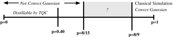
Figure 1. Properties of the state ϱa8(p) = (1 − p)|a8〉〈a8| + pI/16. Our results show that p*, the noise threshold above which ϱa8(p) is convex-Gaussian, is in the interval ![$[\frac {8}{15}, \frac {8}{9}]$](https://content.cld.iop.org/journals/1367-2630/15/1/013015/revision1/nj444794ieqn82.gif) , depicted in gray. In this interval we do not yet know whether ϱa8 is convex-Gaussian. For p < 0.40, Bravyi [2] showed that ϱa8 can be distilled by noiseless braiding operations to enable topological quantum computation (TQC) with Clifford group elements (for quantum universality, one also needs a sufficiently low-noise |a4〉 ancilla). Our results from the SDP on the existence of a Gaussian-symmetric extension of ϱa8(p) for p ⩾ 0.25 do not provide additional information beyond these analytical results.
, depicted in gray. In this interval we do not yet know whether ϱa8 is convex-Gaussian. For p < 0.40, Bravyi [2] showed that ϱa8 can be distilled by noiseless braiding operations to enable topological quantum computation (TQC) with Clifford group elements (for quantum universality, one also needs a sufficiently low-noise |a4〉 ancilla). Our results from the SDP on the existence of a Gaussian-symmetric extension of ϱa8(p) for p ⩾ 0.25 do not provide additional information beyond these analytical results.
Download figure:
Standard imageIn order to give a lower bound on p* we implemented the SDP program 1 for fixed n = 2 (see appendix B) with the aid of the cvxopt library for Sage [34]. The numerical results indicate that p* ⩾ 0.25, as it is always possible to find a Gaussian-symmetric extension for ϱa8(p) with n = 2 for noise rates above this value. Our implementation of the feasibility SDP takes approximately one day for each value of p in a computer with 2.3 GHz processor, and takes about 30 GB of RAM memory. The implementation of the SDP with an additional PPT condition on the extension is likely to provide stronger results, but it is more computationally intensive. Given these limitations, we provide an alternative analysis of the properties of ϱa8(p) using the notion of witnesses: Hermitian operators which have expectation values in a restricted range (e.g. non-negative for all Gaussian states) whereas expectation values on non-Gaussian states can extend beyond this range (e.g. be negative). The existence of such witness operators is guaranteed by the fact that they represent hyperplanes separating the convex-Gaussian states from all even Hermitian operators in  (in addition, similarly as in [29], witnesses could be constructed based on a negative output of feasibility SDP).
Clearly, such Hermitian witness operators, say W, should include terms which are quartic or higher-weight correlators, as the expectation value of quadratic Hamiltonians only depends on the correlation matrix of a state. For ϱa8(p) the obvious choice for such a witness operator is W = |a8〉〈a8|, for which  . Let us understand how we can bound
  where ψg is any Gaussian pure state. We will use the fact that the correlation matrix of |a8〉 is the null matrix, i.e. for all Majorana operators ci,cj, Tr cicj|a8〉〈a8| = 0, which follows directly from equation (17). We will now prove that
  which shows that for
  , the state ϱa8(p) is not convex-Gaussian. The following proposition proves our claimed bound and can be intuitively understood by interpreting the state |a8〉 as a maximally entangled state while Gaussian states are product states:
Proposition 3. For all Gaussian pure states |ψg〉, we have  .
.
Proof. Let c1 and c2, c1c2 = −c2c1, be two arbitrary Majorana fermion operators, from a complete set {c2k−1,c2k}4k=1 (note the SO(8) freedom in choosing these). Let |x〉 denote an eigenvector of the mutually commuting operators ic1c2, ic2k−1c2k for k = 2,...,4 where the bits (0 or 1) of x label the eigenvalues (resp. +1 and −1) of these operators. The Gaussian states |x〉 form a basis for the four-fermion (or four-qubit) space; hence we can write  with
with  . Then

This, together with normalization, implies that  , hence for all y, |α0y|2 and |α1y|2 are less than or equal to 1/2. □
A tighter bound than the one in proposition 3 cannot be excluded if one uses further properties of the state |a8〉—such a tighter bound would lead to a reduction of the gray area in figure 1.
To give an upper bound on p* we construct explicit Gaussian decompositions of ϱa8(p) for large values of p. To do this we consider a subset of the convex-Gaussian states that share some key properties with ϱa8(p), namely: (i) zero correlation matrix, and (ii) only a small fraction of all possible correlators has non-zero coefficients.
To exploit these symmetries we define three types of states:

where ϱMi(λ), for i = 1,2,3, is the Gaussian state generated by the correlation matrix Mi(λ), with λ∈[ − 1,1]4, and Mi(λ) assumes one of the following three forms:

By construction, these states are convex-Gaussian, have null correlation matrix, and any convex combination of them has an expansion in terms of Majorana operators with non-vanishing coefficients only on the same correlators as ϱa8(p). The aim is to find for which p's it is possible to decompose ϱa8(p) as a convex sum of these types of convex-Gaussian states.
In order to describe the convex hull of these states, first note that M2 and M3 are related to M1 by permutations (different choices of pairings):

where

Given that the transformation connecting the correlation matrices is formed by the direct sum of identical permutations, this transformation is in SO(8)—one always gets the signature of the permutation squared, and therefore the corresponding determinant is always 1. Rotations in SO of the correlation matrix induce unitary transformations on the level of the states [19]: P12↦U2, P13↦U3. Bearing in mind this connection among the three classes of states above, we now determine the extreme points of the set of type 1 states.
(Extreme points for type 1 states).Lemma 3 Let ![$\overline {{\mathcal {S}}}_1 = {\mathrm { conv}}\{\varrho _1(\lambda ) | \lambda \in [-1,1]^4\}$](https://content.cld.iop.org/journals/1367-2630/15/1/013015/revision1/nj444794ieqn92.gif) . Then the extreme points of
. Then the extreme points of  are given by

with x∈{0,1}4 and ¬x is the bitwise negation of x.
Proof. It follows immediately from the expansion of the state ϱ1(λ):

□
Defining in a similar fashion  ,
,  , ϕ2(x) and ϕ3(x), we can then define the convex hull of any convex combination of the three types of states as
  . More explicitly,

where the summation in x is to be carried out over its binary expansion in three bits.
The problem now reduces to determining for which values of p∈[0,1] the linear system  , with {γi} a probability distribution, has a solution. Simple inspection shows that such a Gaussian decomposition is always possible whenever p ⩾ 8/9 ≈ 0.89, which is then an upper bound on p*.
5. Discussion: classical simulation of fermionic quantum computation
In contrast to bosonic linear optics, quantum computations based on FLO can be efficiently simulated by a classical computer even when augmented by measurements of fermionic number operators [18–20]. The simulation relies on the following facts
- (i)Efficient encoding of Gaussian states—a Gaussian state of 2m Majorana fermions is fully described by its correlation matrix M, with O(m2) elements.
- (ii)FLO transformations map Gaussian states onto Gaussian states, with an efficient update rule—every FLO transformation
 induces a rotation R∈SO(2m) on the Majorana operators space, . This, in turn, induces the map M↦RMRT
on the 2m × 2m correlation matrix, and this update can be evaluated in O(m3) steps.
induces a rotation R∈SO(2m) on the Majorana operators space, . This, in turn, induces the map M↦RMRT
on the 2m × 2m correlation matrix, and this update can be evaluated in O(m3) steps. - (iii)Efficient read-out of measurement probability distributions—via Wick's theorem (6) the probability of measuring the population in fermionic modes can be done efficiently, as the Pfaffian of a 2m × 2m matrix can be evaluated in O(m3). Furthermore, number operator measurements project Gaussian states onto Gaussian states.


With these three ingredients, the evolution of any initial Gaussian state can be efficiently followed by a classical computer at any time in the computation, and the output distribution can be exactly evaluated. In [19, 21], the allowed transformations in (ii) were extended to noisy Gaussian maps. These are completely positive channels, not necessarily FLO unitaries, that map Gaussian states onto Gaussian states, and as such still admit efficient classical simulation.
Our results imply that if p ⩾ 8/9, ϱa8(p) is convex-Gaussian and this allows for the classical simulation of the computation as follows. Given a noise strength p ⩾ 8/9, one finds the decomposition of ϱa8(p) in  , by solving the linear system
  —this has to be done only once for a fixed p. As each ϕi(x) is in itself a convex sum of two pure Gaussian states, this leads to a decomposition of ϱa8(p) in terms of at most 48 pure Gaussian states. Let pi be the probability associated with the ith pure Gaussian state in such a decomposition. Then, whenever a state ϱa8(p) is requested in the computation, one samples from {pi} and chooses the corresponding pure Gaussian state. From this point onwards, the simulation follows the scheme summarized in (i), (ii) and (iii) above.
The results in figure 1 leave some gaps in our understanding, in particular about the precise value of p*. In order to improve the lower bounds on p* one could consider distillation processes beyond the restricted set of braiding operations, but that still map Gaussian states onto Gaussian states, leaving thus the set of convex-Gaussian states unchanged. The distillation protocol of depolarized GHZ4 states, which are isomorphic to ϱa8(p), proposed by Dür and Cirac at first sight suggests that our classical simulation threshold is tight, as it can distil a perfect GHZ4 provided that p < 8/9. Nevertheless, their protocol uses non-FLO operations, as it assumes that one can locally create the GHZ4 and uses distilled two-qubit maximally entangled pairs for distribution. The protocol devised by Murao et al in [35] directly distils GHZ4 from depolarized copies of it for p < 0.7328. Despite the fact that this direct approach seems more related to our question, it employs gates that are not immediately translated into braiding operations or even to FLO transformations. Although the choice to distil via braiding operations is physically motivated—due to their topological protection—a different distillation threshold from FLO operations would suggest that either Bravyi's distillation protocol can be improved to higher depolarizing noise rates or that there exists a 'transition zone' in which the computation by braiding of Majorana fermions is neither quantumly universal nor can be efficiently simulated classically.
Acknowledgments
We acknowledge fruitful discussions with Akimasa Miyake, Ronald de Wolf, Sergey Bravyi and Volkher Scholz. We also thank Maarten Dijkema for IT support. Fd-M is supported by the Vidi grant 639.072.803 from the Netherlands Organization for Scientific Research (NWO).
Appendix A.: Symmetric versus Gaussian-symmetric subspace
Inspired by [36], we define a 'FLO twirl' as the map  where
where  is defined by taking the Haar measure over the real orthogonal matrices R induced by U. The map
  is normalized such that it is trace-preserving.
Lemma A.1. The projector onto the null space of  is
is  where |0〉 is a (Gaussian) vacuum state with respect to some set of annihilation operators ai. Thus the states |ψ,ψ〉 where ψ is a pure fermionic Gaussian state span the null space of Λ, which implies that the null space of Λ is a subspace of the symmetric subspace.
Proof. In order to prove that  , we note that both the lhs and the rhs are U⊗U-invariant where U is any FLO transformation. Thus instead of considering whether
  for any X, we can just consider the trace with respect to invariant objects
  . It can be shown that Λi for i = 0,1,2,...,2m (and linear combinations thereof) are the only invariants under the group U⊗U where U is FLO transformation [37].9 Clearly,
  for all i ≠ 0 while
  fixes the overall prefactor. Having established the form of the projector, it follows directly that the states |ψ,ψ〉 for any Gaussian ψ span the null space. (Assume that this is false and hence a state in the null space |χ〉 = |χin〉 + |χout〉 where |χin〉 is in the span of |ψ,ψ〉 while |χout〉 is w.l.o.g. orthogonal to any |ψ,ψ〉. We have ΠΛ=0|χ〉 = |χ〉 while
  arriving at a contradiction.) As |ψ,ψ〉 for Gaussian pure states ψ span the null space, and P|ψ,ψ〉 = |ψ,ψ〉 with P the SWAP operator, the null space is a subspace of the symmetric subspace. □
Appendix B.: SDP for detecting non-convex-Gaussian states
Recall the series of tests constructed to detect if a state  is not convex-Gaussian:

Note that we have explicitly kept the permutation-symmetry constraint in this program.
In this appendix, we convert this problem into a feasibility semi-definite programming problem. To do that we must show that the above problem can be cast as the standard form of SDPs, namely

where  is the unknown vector to be optimized over, c is a given vector in
  , and {Fi}i=0,...,d are given symmetric matrices. For the equality constraint,
  is a given matrix, with rank(A) = p, and
  . The restriction on the rank of A demands that the linear system has at least one solution, and all the rows are linearly independent.
The first step is to associate an Hermitian operator Mj with each term ikca1ca2···ca2k in the expression (1). The set {Mj}0⩽j⩽22m−1−1 spans all the even Hermitian operators of  . Then any state
  can be written as

and we choose M0 = I.
For definiteness, in what follows we restrict ourselves to the case n = 2. Extensions to larger n follow the same structure and can be immediately constructed. That said, a general extension on  can be written as

with the coefficients  to be fixed by the constraints of our problem. The symmetry constraint can be taken directly into the parameterization of ϱext by imposing that

At this point, the initially 24m−2 coefficients of ϱext are reduced to 22m−2(1 + 22m−1).
The imposition that Tr1(ϱext) = ϱ further demands that

Therefore, β0,j = αj/2m. In this way, a further 22m−1 coefficients are determined, and thus there remain 22m−3(22m − 2) free parameters. Note that the normalization of ϱext is already guaranteed as long as Tr(ϱ) = α0 = 1.
The question of whether there exists an assignment of the remaining free coefficients respecting the last two constraints can be immediately posed as a feasibility SDP:

Forgetting for the moment that the correlators are in general complex, a direct correspondence with the SDP standard form can be done as follows:


with x = ({βj,j}1⩽j⩽22m−1−1,{βj,k}1⩽j<k⩽22m−1−1)T.
The equality constraint then reads

This can be cast in the form Ax = b, by writing A = ([ΛFi]1⩽i⩽22m−3(22m−2)) and b = −[ΛF0]. The notation [G] means a column matrix constructed by stacking each column of G below each other.
To finish the construction we must take into account that we are possibly dealing with complex values. To do that we employ the following well-known result.
Lemma B.1. Let  . Then Z ⩾ 0 iff
  .
.
Proof. (⇒) Let z = x + iy be an eigenvector of Z with eigenvalue λ. Then it is easy to see that (x,y)T is an eigenvector of  with eigenvalue λ.
(⇐) By the same token, let (x,y) be an eigenvector of  with eigenvalue λ. Then z = x + iy is an eigenvector of Z with eigenvalue λ. □
The final dimension of each Fi is then 22m+1 × 22m+1, and there are 22m−3(22m − 2) of such matrices. For the equality constraint we write

The final matrix (Re(A), Im(A))T has dimension 24m+1 × 22m−3(22m − 2). Most likely, the rank of this matrix is not equal to the number of rows. Therefore, before plugging it into the SDP one must evaluate its reduced-row form (echelon form), and remove the all-zero lines.
If one wishes to include the PPT test, as in program 2, this can be done by rewriting the two positivity constraints, ϱext ⩾ 0 and ϱT1ext ⩾ 0, as a single one, ϱext⊕ϱT1ext ⩾ 0. One thus needs to map each complex Fi in the positivity constraint to F'i = Fi⊕FT1i. The final dimension of each real F'i is then 22m+2 × 22m+2. The equality constraint remains the same.
Footnotes
- 4
Non-interacting fermionic operations are unitary transformations generated by quadratic Hamiltonians on the creation and annihilation operators of fermionic modes. Such Hamiltonians can always be block-diagonalized, and in this new basis the different fermionic modes do not interact.
- 5
Any Gaussian fermionic state with an even number of fermions can be brought, by fermion-number preserving quadratic interactions, to a normal form which is a superposition of states with fixed pairs of fermions created from the vacuum, see e.g. [13].
- 6
A system of m qubits is isomorphic with a system with m fermions and the unitary Jordan–Wigner transformation maps each Majorana fermion operator onto a non-local product of Pauli operators acting on m qubits.
- 7
Let A = (ai,j) be a 2m × 2m anti-symmetric matrix; then
, where S2m is the set of all permutations of 2m symbols. The Pfaffian is non-zero only for an anti-symmetric matrix of even dimension. - 8
Adding the permutation symmetry would of course leave the program in SDP form.
- 9
