


Abstract
An exact solution is derived for the wavefunction of an electron in a semiconductor quantum wire with spin–orbit interaction and driven by external time-dependent harmonic confining potential. The formalism allows analytical expressions for various quantities to be derived, for example spin and pseudo-spin rotations, energy and occupation probabilities for excited states. It is demonstrated how perfect spin and pseudo-spin flips can be achieved at high frequencies of the order of ω, the confining potential level spacing. By an appropriately chosen driving term, spin manipulation can be exactly performed far into the non-adiabatic regime. The implications for spin-polarized emission and spin-dependent transport are also discussed.
Export citation and abstract BibTeX RIS

Content from this work may be used under the terms of the Creative Commons Attribution-NonCommercial-ShareAlike 3.0 licence. Any further distribution of this work must maintain attribution to the author(s) and the title of the work, journal citation and DOI.
One of the first proposals for the solid-state realization of quantum information processing and computation is based on the use of the spin degree of freedom of electrons, confined in quantum dots (QD), which realize the qubit [1], and several universal quantum computation propositions [2–4] have been deduced from this basic idea.
Experimental progress in measurements and coherent manipulation of electrons in QD systems has been immense in recent years [5–17]. Coherent single-electron spin rotations have been realized using oscillating magnetic [5] and oscillating electric fields [6, 7]. A limitation of these schemes is the long single-spin rotation times, of the order of tens of ns. By exploiting ultrafast laser control and optical pumping, single-spin control was demonstrated on a ps timescale [8, 9]. All electrical two-qubit gates composed of single-spin rotations and interdot exchange in a double QD were also demonstrated [10]. By using surface acoustic waves, single electrons have been transfered between QD separated by a few μm [11, 12], where McNeil et al [12] have reliably relocated a single electron back and forth between the dots multiple times up to a cumulative distance of 0.25 mm. Controlled production of entangled qubit pairs in QD and surface acoustic waves was predicted theoretically [18–20]. The coherent time evolution of single-electron charge dynamics on a time scale of a few picoseconds was measured [13]. Tunable non-adiabatic single-electron excitations were observed recently [14], where a rapid modulation of the confining potential causes transitions to excited orbital states.
Due to the lack of inversion symmetry in semiconducting materials, the electron spin is coupled to the orbital motion [21, 22]. Rather than treating this interaction as a source of decoherence, it can be harnessed to coherently manipulate spin-orbital qubits [4, 7, 23–28]. The rotation of a spin-orbital qubit in a moving quantum dot has been studied analytically in the adiabatic limit. Single-qubit manipulation, spin-flip for example, can easily be performed by adiabatic spatial QD translation for a distance of the order of the spin–orbit length [24–27]. However, the condition of adiabaticity sets a severe upper limit for the speed of single-qubit operations. Although an analysis by means of a full numerical simulation is possible, it gives results only for particular cases and the optimization and elimination of errors is not straightforward [27].
In this paper, we extend analytic results for spin manipulation by the adiabatic translation of a QD [24–26] to include the non-adiabatic regime, thereby opening up the possibility of much faster spin–qubit rotations. In particular, we analytically solve the one-dimensional (1D), non-adiabatically driven QD with harmonic confining potential in the presence of spin–orbit interaction. Although it is demonstrated how a general solution can be constructed, we also present explicitly four typical driving schemes with a focus on the non-adiabatic regime. The system considered here is similar to the one presented by Flindt et al [23], where the authors performed a spin-flip by displacement of a QD in a wire. Such a system has even been realized experimentally [7, 28–31], with the ability to control a single electron, in InAs [30] and Ge [31] quantum wires. More recently, spin–orbital qubits in double QD have also been demonstrated in InSb quantum wires [28].
The 1D Hamiltonian we consider is given by

where an electron with an effective mass m* is confined in a harmonic trap with frequency ω, centred around the time-dependent position of the harmonic potential minimum ξ(t), α and β are the Rashba [21] and Dresselhaus [22] spin–orbit couplings, respectively, and we use units with ℏ = 1 throughout the paper.
First we apply the unitary transformation

which consists of a canonical transformation that eliminates the spin–orbital part of the Hamiltonian [32],

and of the part which eliminates the time-dependent part of the Hamiltonian [33],
Here xc(t) is the solution of the equation of motion for a classical particle in a driven harmonic oscillator potential,

for xc(0) = 0 and  customarily given by
 ![$x\mathrm {_c}(t)=\omega \int _0^t \sin [\omega (t-t')] \, \xi (t') \, \mathrm {d}t'$](https://content.cld.iop.org/journals/1367-2630/15/1/013029/revision1/nj444234ieqn2.gif) .
.
The original time-dependent Schrödinger equation i ∂t Ψ = H(t) Ψ is transformed into

where ψ = U(t) Ψ. The transformed Schrödinger equation takes the form of a static harmonic oscillator

with an energy shift Eso = −m* (α2 + β2)/2. In deriving equation (7) some care is needed in showing that terms in iU(t)∂tU†(t) precisely cancel the counterparts in U(t)H(t)U†(t). The solutions of the original Hamiltonian (1), Ψns(x,t), with the initial condition Ψns(x,0) = e−S ψn(x) χs, where ψn(x) is the nth eigenfunction of the undriven harmonic oscillator (7) and χs is a spinor with spin s, are obtained directly via the unitary transformation (2), i.e.

where  is a phase factor and ωn = (n + 1/2)ω.
From the exact time-dependent solution, (8), we see that the effect of non-adiabatic motion is to displace the harmonic oscillator eigenstate wave packet away from the quantum-dot minimum at ξ(t) to a new position xc(t), given by the solution of the classical oscillator, (5). It is clear that this will excite the electron in the QD, and explicit calculation gives
where Ec(t) is in fact the classical expression for the harmonic oscillator energy.
To simplify the analysis, we consider quantum wires grown in the [111] direction, for which β = 0. For this case, the mean spin rotates around the y-axis by an angle 2 xc(t)/λso, where λso = (m* α)−1, following immediately from equation (8), from which the expectation values of the spin components may also be evaluated explicitly. For example, if the initial state is the pseudo-spin-up Kramers state, Ψ0↑(x,0) = e−i x/λso σy ψ0(x) χ↑, the spin expectation values are
where the oscillatory factors are consistent with the mean spin rotation and the decaying exponential factors account for the spread in the wavefunction, which is given by σ = (m*ω)−1/2. Due to the precession of spin around the y-axis,  is constant and zero for our choice of the initial state.
In figure 1(b), we show specific choices of the driving term, ξ(t), for the cases when the transit time, T, is chosen to give a perfect spin-flip, for which the dot displacement is πλso/2. The detailed results for these choices and general T are given below. Here we note that, in general, there will be residual oscillations of the electron distribution after the dot stops, leading to uncertainty of the order of 2 a/λso in the spin rotation angle, where a is the amplitude of the residual orbital oscillations and the final energy is given by  . Such residual oscillations of the electron wave packet after the dot has stopped will also give rise to orbital decoherence through phonon emission and subsequent spin decoherence via the spin–orbit interaction. However, it is clear that ξ(t) can always be chosen such that these residual oscillations are totally suppressed with the wavefunction returning to the centre of the QD and remaining there, i.e. xc(t) = ξ(T) and
  for all t > T. This is a very physical result which can be understood in purely classical terms from equation (5).

Figure 1. (a) Schematic view of a semiconductor quantum wire deposited on gate electrodes which provide a time-dependent harmonic potential. Such systems have been realized experimentally [7, 28, 29]. (b) The position ξ(t) of the harmonic potential minimum. After driving time T the QD stops at displacement ξ(T). The black line corresponds to the fastest unidirectional QD translation, with a minimum spin-flip time T0/2, where T0 = 2 π/ω and ω is the confining potential level spacing. In addition to instantaneous displacement, the other drivings considered are: linear ramp with ξ(t) = ξ(T)t/T (blue dashed) and sinusoidal with ![$\xi (t) = \xi (T)\, \bigl [ t/T \pm \, \sin (2 \, \pi \, t/T)/(2 \, \pi ) \bigr ]$](https://content.cld.iop.org/journals/1367-2630/15/1/013029/revision1/nj444234ieqn7.gif) (green dot-dashed and red solid), giving spin-flip times of T0,
(green dot-dashed and red solid), giving spin-flip times of T0,  and 2 T0, respectively.
Download figure:
Standard imageA further interesting general observation is that under forced oscillations in which the quantum dot is translated back and forth non-adiabatically in one dimension, energy will be transferred to the electron wave packet in the dot, and under resonant conditions the amplitude of the displacement of the classical oscillator (and hence the position of the wavefunction relative to the potential minimum) will increase, as will the mean energy of the electron given by equation (9). These oscillations will be accompanied by a corresponding rotation of the spin which will also have oscillatory components, due to the oscillation of the dot and the oscillation of the wavefunction relative to the dot. It would be interesting to observe the effects of these oscillations experimentally, e.g. in the polarization distribution of radiative emission when the excited electron in the quantum dot relaxes or by using a weak repeated measurement of the current [13, 14].
In materials with spin–orbit interaction, in addition to the real spin, one can also study the pseudo-spin, defined by
where  are the eigenstates of the potential at a particular instant t,

For the initial Kramers pseudo-spin-up state,  , a straightforward calculation leads to a simple exact expression for the expectation value,
and  . Pseudo-spin is dependent only on the position of the QD; therefore slow adiabatic or arbitrary fast non-adiabatic motion leads to identical pseudo-spin values. Furthermore, the pseudo-spin is independent of the spread in orbital wavefunction, being a composite of spin and orbital degrees of freedom. In the derivation of this result, we express the coefficients in the instantaneous basis given by (12),
where  , with
 ![$\eta\kern-1pt=\kern-1pt-m^*\dot{x}_{c}(t)^2/(2\omega)+{\rm i}m^*\dot{x}_{c}(t)[x_c(t)-\xi(t)]/2$](https://content.cld.iop.org/journals/1367-2630/15/1/013029/revision1/nj444234ieqn13.gif) , is the overlap of the nth eigenfunction of the quantum harmonic oscillator and the ground state displaced by
, is the overlap of the nth eigenfunction of the quantum harmonic oscillator and the ground state displaced by  , which gives
 ![$\langle n \bigl | 0 \rangle _d = [d/(\sqrt {2} \sigma )]^n \exp [- |d|^2/(4 \, \sigma ^2)]/\sqrt {n!} \,$](https://content.cld.iop.org/journals/1367-2630/15/1/013029/revision1/nj444234ieqn15.gif) . Therefore
. Therefore  is a coherent state and the probability for occupation of the nth manifold is given by the Poisson distribution,
 ![$P_n(t)=\sum _{\mathrm {s}} |c_{n s}(t)|^2= [E_{\mathrm {c}}(t)/\omega ]^n\exp [-E_{\mathrm {c}}(t)/\omega ]/n!$](https://content.cld.iop.org/journals/1367-2630/15/1/013029/revision1/nj444234ieqn17.gif) .
.
From equation (14), we see that the exact wavefunction at time t may be written as
where  . In this form, we see explicitly the rotation of the pseudo-spin on the Bloch sphere and also the time dependence of the orbital part of pseudo-spin states
  .
.
Pseudo-spin qubits in systems with strong spin–orbit interaction are usually restricted to the manifold spanned by the ground-state Kramers doublet, as studied in [7, 23–27]. Pseudo-spin (11) is in this case limited to the n = 0 manifold. For the initial Kramers pseudo-spin-up ground state Ψ0↑(x,0), the expectation value of pseudo-spin is related to the probabilities  and
and  that the system is in the ground state with pseudo-spin up or down, respectively.
Direct evaluation gives  , where P0↑ = P0 cos2(ξ/λso) , P0↓ = P0 sin2(ξ/λso) , which leads to

Note that in the adiabatic limit, the moving electron remains at the potential minimum, i.e. xc(t) → ξ(t) and Ec(t) → 0, and the pseudo-spin coincides—up to an exponential factor due to a wavefunction spread—with the real spin, given by (10).
To be specific, we examine four examples of the driving term ξ(t): sudden displacement in two steps, a constant velocity of the QD displacement and two different types of smooth driving with sinusoidal (ac) type velocity, as shown in figure 1(b). In all cases, the QD stops moving after the transit time T. Then, the position expectation value oscillates with the amplitudes of residual oscillations a, as follows from the classical solution xc(t) of the equation of the motion (5). For example,
for the constant velocity (ac) case and the smooth sinusoidal case (as), as introduced in figure 1 (blue dashed and red full, respectively).
The shortest time with no residual oscillations for unidirectional movement of the dot, Tmin, is achieved by instantaneous displacement of the dot for π λso/4, followed by a waiting time T0/2, followed by another instantaneous displacement for π λso/4. For any other unidirectional driving the minimum time Tmin rises. In the limit T → 0 all unidirectional movements of the dot lead to oscillations with the amplitude ξ(T) = π λso/2. In figure 2(a), residual oscillations are presented as a function of driving time T. In all cases, the residual oscillations vanish when some resonant condition for T/T0 is fulfilled. The oscillations are proportional to the spin–orbit length λso and have a simple dependence on T0 and T. As expected, smooth sinusoidal driving exhibits significantly fewer residual oscillations compared to the other forced oscillations considered. As demonstrated here, by using the solution to a classical driven harmonic oscillator we gain insight into a driven QD in a semiconducting nanowire.
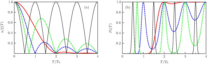
Figure 2. (a) The amplitude of residual oscillations after the QD stops, ![$a=\sqrt {[x_{\mathrm {c}}(T)-\xi (T)]^2+\dot {x}_{\mathrm {c}}(T)^2/\omega ^2}$](https://content.cld.iop.org/journals/1367-2630/15/1/013029/revision1/nj444234ieqn23.gif) , divided by the QD displacement ξ(T) = π λso/2 for drivings as in figure 1(b): the fastest unidirectional driving (black full), constant velocity (blue dashed) and the two sinusoidal drivings, a broken (green dot-dashed) and a smooth one (red full). (b) Probability for the ground-state doublet occupation after the QD stops. We use material parameters typical of InSb [28] given by m* = 0.015me, where me is the electron mass, λso = 150 nm and the confining potential level spacing ω = 10 meV. This gives σ = 0.1 ξ(T).
, divided by the QD displacement ξ(T) = π λso/2 for drivings as in figure 1(b): the fastest unidirectional driving (black full), constant velocity (blue dashed) and the two sinusoidal drivings, a broken (green dot-dashed) and a smooth one (red full). (b) Probability for the ground-state doublet occupation after the QD stops. We use material parameters typical of InSb [28] given by m* = 0.015me, where me is the electron mass, λso = 150 nm and the confining potential level spacing ω = 10 meV. This gives σ = 0.1 ξ(T).
Download figure:
Standard imageIn figure 3(a), the z-component of spin after one cycle is presented for linear ramp and smooth sinusoidal driving for T/T0 = 2 and 5. For this spin-flip case the quantum dot is displaced for a distance ξ(T) = π λso/2. Note that the magnitude of  does not quite reach
  at the beginning and end of the spin-flip due to the spread in the Gaussian wavefunction, which gives
  from equation (10). Note also the weak oscillation superimposed on the cosine curve which, again, can be understood directly from the exact solution, equation (10), which shows a perfect cosine variation when plotted against xc rather than ξ. For xc − ξ small, we may expand to lowest order giving cos(2xc/λso) = cos(2ξ/λso) − 2 (xc − ξ) sin(2ξ/λso)/λso, which is the form shown in the figure, since xc − ξ has n = T/T0 oscillations. These oscillations are both positive and negative with respect to the adiabatic limit (black full line), which shows a perfect cosine (also with amplitude attenuated by the Gaussian factor in equation (10)) but with no superimposed oscillation since ξ(t) = xc(t) for all t. It should be additionally stressed that for non-resonant values of T/T0, there will be residual oscillations as shown in figure 2(a) and the spin expectation values (10) will continue to oscillate after the dot stops.

Figure 3. (a) The z-component of the spin expectation value as a function of QD displacement in the non-adiabatic regime for two types of driving. The black full line represents the adiabatic limit (T → ∞). Note the oscillations superimposed on the cosine curve giving rise to both positive and negative fluctuations in mean spin relative to the adiabatic limit. (b) Ground-doublet pseudo-spin expectation,  , for the same parameters as in (a). Note that
  precisely and that the effect of non-adiabaticity leads to greater deviation from cosine (compared with real spin) at intermediate times, which is always suppressed due to breakdown of the ground-doublet approximation. (c) Typical probability for occupation of the ground state doublet during the driving (sinusoidal), P0(t), in the non-adiabatic regime. The arrow indicates the direction of increasing T (T/T0 = 2, 2.5, 3.5, 4.5, 6.5); bullets indicate minimum values P0min. (d) P0min as a function of T/T0; bullets are as in (c). All parameters are the same as in figure 2(b).
Download figure:
Standard imageIn figure 3(b), the ground-doublet pseudo-spin expectation  is presented for the same conditions as in (a). The adiabatic limit (black full line) is now a perfect cosine with amplitude
  , and this is also the result for full pseudo-spin
  for any T consistent with spin-flip (see equations (11) and (13)). On the other hand, we see that there are significant deviations for non-adiabatic motion in the ground-doublet approximation, signalling its breakdown due to suppressed probability of ground-doublet occupation and corresponding suppression of
  relative to the adiabatic limit. These deviations do not occur, however, at the beginning and end of the spin-flip for which the function ξ(t) has been chosen so that the electron starts and ends in its ground-doublet located in the centre of the dot. Nevertheless, we see from figures 3(a) and (b) that any error in the total displacement will give spin-flip errors that are significantly smaller for the smooth sinusoidal choice of ξ(t), as expected.
For all the different driving functions ξ(t), the optimum spin (or pseudo-spin) transformations, which leave the electron in its lowest energy state after the transit of the dot, may always be determined. Such states depend only on the distance the dot travels, independent of the degree of non-adiabaticity, provided that the motion is coherent. However, the states of the electron in the dot at intermediate times/distances do depend strongly on the degree of non-adiabaticity and a convenient measure of this is the deviation from unity of the probability for the ground state, P0. For t ⩾ T this probability is simply determined by the residual oscillations, P0(T) = e−a2/(2 σ2), as shown in figure 2(b) for driving functions as in figure 2(a). In figure 3(c), the time dependence of P0(t) for different values of T/T0 is presented for the smooth sinusoidal case: for large T, P0 ∼ 1, while for short times the minimum of P0 = P0min around t ∼ T/2 signals the increase in probability for exciting higher energy states. The transition from the highly non-adiabatic to the adiabatic regime is clearly seen also from the behaviour of the minimum value of P0, plotted in figure 3(d), which at high T monotonically reaches the unitary limit.
In a realistic quantum dot, deviations from a harmonic confining potential will occur at high energy for which the solutions given by equation (8) will be in error. However, as long as the energy at which anharmonic deviations become important is higher than the driving energy, the higher (non-harmonic) excited states will have only a small probability of occupation. The solution presented in this paper will then be a good approximation and the probability of excited-state occupation will still be given by the Poisson distribution to high accuracy. Another source of error will be thermal occupation of excited states when the temperature is higher than the energy level spacing ω. Within the harmonic approximation the results presented here may be extended to take into account thermal occupation of the initial state using a density matrix. The time evolution may then be determined using the exact solution, equation (8), for each harmonic component.
To conclude, we have presented exact solutions of an electron in a driven QD in a 1D quantum wire with spin–orbit interaction. The solutions can be expressed analytically for a broad class of driving schemes. The essence of the full quantum mechanical solution is in the solution for the corresponding classical harmonic pendulum and together with the application of the appropriate canonical transformation. Exact analytical formulae for spin, pseudo-spin, average energy and probabilities for the occupation of excited states are given in terms of the coordinates of the QD and the position of the corresponding classical pendulum. To be specific, we mainly focused on two typical driving regimes: a constant velocity and a smooth sinusoidal driving—in both cases in the full range from adiabatic to non-adiabatic driving. We demonstrated that perfect spin-flip can be realized even in the far non-adiabatic regime, providing driving which by virtue of the formalism can easily be appropriately tuned. The solution given here may be used to guide more complicated simulations for the design of realistic gated device structures.
Two extreme non-adiabatic regimes were highlighted. The first is when the forced oscillator is chosen such that after the transit time of the quantum dot the wavefunction of the electron is at the bottom of the QD potential well and remains there. The main advantage of this choice is that the associated spin rotation (single-qubit transformation) may be determined with maximum precision and does not subsequently change with time. The other extreme regime is exactly the opposite in which the forced oscillations have maximum amplitude after the transit time (resonance). Indeed, we can increase this amplitude indefinitely using a periodic driving term for the dot motion when it is resonant with the harmonic oscillations of the electron in the QD. The amplitude of these oscillations will, of course, be ultimately limited by dissipative processes, in particular, phonon and radiative emission, although in clean systems coherent oscillations should survive to large amplitudes. What is special about such systems is the intimate connection between the motion of the dot, the electron probability distribution relative to the dot and spin rotation. It would be an interesting challenge to observe the effects of such charge-spin oscillations experimentally, for example in spin-polarized emission or spin-dependent transport.
Acknowledgments
The authors thank T Rejec for discussions and acknowledge support from the Slovenian Research Agency under contract no. P1-0044 and the EU grant NanoCTM.