


Abstract
We propose a calorimetric measurement of work in a quantum system. As a physical realization, we consider a superconducting two-level system, a Cooper-pair box, driven by a gate voltage past an avoided level crossing at charge degeneracy. We demonstrate that, with realistic experimental parameters, the temperature measurement of a resistor (environment) can detect single microwave photons emitted or absorbed by the two-level system. This method would thus be a way to measure the full distribution of work in repeated measurements, and to assess the quantum fluctuation relations.
Export citation and abstract BibTeX RIS

Content from this work may be used under the terms of the Creative Commons Attribution 3.0 licence. Any further distribution of this work must maintain attribution to the author(s) and the title of the work, journal citation and DOI.
To define the work performed on a driven quantum system in a physically sound way has turned out to be a truly non-trivial task, except in some special cases of limited applicability [1–12]. This topic has been the focus of intense research recently in the attempts to generalize the classical fluctuation relations [13–18] into the quantum regime. Here we propose and demonstrate that a calorimetric measurement gives both a theoretical and experimental tool to test the Jarzynski equality (JE) and other fluctuation relations in an open quantum system, and to analyze the distribution of dissipation in them, based on the very principle of conservation of energy. We focus on an experimentally feasible two-level system, a superconducting Cooper-pair box (CPB) [19–21] subject to Landau–Zener (LZ) interband transitions [22–24]. Because of the small heat capacity and weak relaxation to the phonon bath, the calorimetric measurement on the electron gas (resistor) turns out to be a very feasible experimental method.
Consider the basic setting for non-equilibrium fluctuation relations [14, 15]: the system is coupled to a bath and is initially in thermal equilibrium with it. Thereafter it is driven by a control field in a non-equilibrium fashion. We are interested in the distribution of work performed on the system in repeated experiments with identical driving protocol among the realizations. In order to secure thermal equilibrium in the next realization, the interval between the repetitions is ideally infinitely long. We mainly consider the protocols where the drive signal returns to its initial position or to an equivalent one with equal free-energy at the end. Our main statement in this respect is then that, due to the energy conservation, the work W done on the system under these conditions is equal to the heat Q dissipated to the environment in the time interval from the beginning of the driving till the end of the equilibration period. With this premise we can avoid the formidable task of analyzing the work itself during the quantum evolution, characterized by difficult-to-analyze time-orderings of the operators involved. The calorimetric principle can, at least in principle, be extended to more general protocols by bringing the system back to the initial position adiabatically at the end of the protocol.
Before going into the detailed analysis of the calorimetric method, let us first define the quantum system and present results in certain limiting cases for the work distribution, which can be obtained by known methods. We focus on a quantum two-level system, shown in figure 1 and characterized by an avoided level crossing under the operation of the control parameter q. For simplicity, we consider a symmetric set-up, where the maximum energy spacing between the ground (g) and the excited (e) level is Emax in the beginning and the end of the drive, and Emin at the minimum in the middle. We normalize q such that it obtains the values ∓1/2 at the beginning and the end of the drive, respectively, and assumes a value q = 0 at the avoided crossing. Suppose for the basic illustration that the system evolves in a unitary way from the initial state: this represents very weak coupling to the environment. In other words, the system is initially thermalized by coupling it to a bath with inverse temperature β, and decoupled from the bath for the duration of the driven evolution. This corresponds to a common situation for considering the fluctuation relations [10, 11, 14]. The value of work in each realization is then determined by the internal energy stored in the system during the operation. There are two possibilities: the system makes an LZ transition around q = 0 between the two states with probability PLZ, or it does not make the transition with probability 1 − PLZ. If the system makes the transition, work ±Emax is done on the system (+ for g → e transition, and − for the e → g transition) by the end of the driving, otherwise the performed work vanishes. The distribution of work W can then be written as

in agreement with the results in [2, 9]. Here δ(E) refers to the Dirac delta function, and ρ0gg = (1 + e−βEmax)−1 is the initial thermal population in the ground state. We may also state that the same distribution as for work applies for heat in the sense discussed above, since after an infinitely long time, for even weak coupling, the system has relaxed back to the thermal equilibrium state by exchanging energy with the environment. Examples of work distributions (with broadening) are shown in figure 1(b) at a few bath temperatures. As for quantum systems evolving unitarily from a thermal state, the JE holds naturally for the two-level system. Indeed we see immediately that

for the distribution of (1). Here the brackets 〈·〉 refer to averaging over the experimental realizations. Equations (1) and (2) simply confirm the earlier understanding of JE in a closed quantum system. The true challenge, which can be addressed by the here-proposed calorimetric detection, is, however, the measurement of work in an open quantum system coupled to the environment also during the driving period.

Figure 1. A two-level system with avoided crossing between the ground (g) and the excited (e) state. In (a) the control parameter q is swept from left to right and the system is initially in the ground state and evolves either in the ground state (probability 1 − PLZ) or makes an LZ transition (probability PLZ). (b) Examples of the distribution of work in repeated sweeps under the conditions that the system starts in thermal equilibrium at various temperatures, and it is not coupled to the environment during the evolution. The distributions correspond to (1) with artificial broadening of the peaks, and for PLZ = 0.3, and βEmax = 0.1,0.3 and 1.0 (red, blue and black curves, respectively). The peak at W = −Emax arises from e to g LZ transitions, the peak at W = 0 is for adiabatic evolution, and that for W = + Emax arises from g to e transitions, as indicated by the diagrams within the (b) panel.
Download figure:
Standard image High-resolution imageAlthough our proposal and arguments are quite general, as will be discussed below, we next specify a particular physical system, a CPB, where concrete results about the distribution of work, and a description and analysis of the calorimetric measurement are immediately possible and can be implemented experimentally. The CPB [19–21] consists of a superconducting island connected to a superconducting lead by a Josephson tunnel junction. The system is described by the circuit scheme in the inset of figure 2 and it is characterized by a voltage source Vg, coupling gate capacitance Cg, a Josephson junction with energy EJ and capacitance CJ. We denote CΣ ≡ Cg + CJ. Resistor R forms the dissipative environment of the box. In the regime  ≡ EJ/(2EC) ≪ 1, where EC = 2 e2/CΣ is the charging energy of the box, we can treat the CPB as a two-level quantum system [21]. Denoting with |0〉 and |1〉 the states with zero and one excess Cooper-pairs on the island, respectively, the Hamiltonian of the system reads

where q = CgVg/(2e) is the normalized gate voltage. We assume a linear gate ramp q(t) = −1/2 + t/τ over a period  starting at t = 0, when the state |0〉 is the ground state of the CPB. The energy gap separating the ground and the excited state of the system is given by
  . Thus the system passes a minimum energy gap Emin = EJ at q = 0, see figure 1(a), where it makes a transition with the probability
  according to the standard LZ model [22–24]. The value of the energy gap at the ends of the trajectory is
  .
.
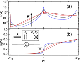
Figure 2. Numerical results of the distribution of work in a CPB. The circuit is shown in the inset of (b). In (a) we present the actual distribution p(W). The parameters of the system are EJ/kB = 0.1 K, EC/kB = 1 K, λ = 0.3, bath temperature (kBβ)−1 = 0.2 K, τ = 1 × 10⁻⁹ s and R/RQ = 1/3,1,10/3,10. Each distribution is based on 9 × 10⁷ repetitions. In (b) we show the corresponding cumulative distributions  with the same coloring of the lines as in (a).
Download figure:
Standard image High-resolution imageWe proceed further by applying the calorimetric principle to an open driven two-level system, the main example being a CPB. Full description of the statistics of the work done and the heat generated by the CPB under the driven evolution with LZ transitions in the dissipative regime is beyond the focus of the present work. We restrict the discussion to the regime when energies on the order of the minimum gap EJ or smaller can be neglected. In this approximation, dynamics of the two-level system can be described by the master equation for probabilities p0 and p1 for the system to be in the charge states |0〉 and |1〉:

with the rates of transitions between these states given by

where E = 2ECq is the energy dissipated to or absorbed from the environment (resistor) in the + (0 → 1) or − (1 → 0) transition, and

is the corresponding probability density of the system to emit energy E to the environment [25]. The standard correlation function in (6) is given by

Here, RQ ≡ ℏ/e2 and the relevant impedance of the CPB reads

where Reff = λ2R, Ceff = CJCΣ/Cg and λ ≡ Cg/CΣ is the coupling parameter. This master-equation-based approach to the description of the system dynamics can be justified most directly in the 'incoherent' regime, when the broadening of the energy levels due to the coupling to environment is larger than EJ. However, as discussed below, it also quantitatively reproduces main results for the coherent LZ dynamics.
As an illustration of this, we consider first the case of vanishing temperature T. In this case, the system dynamics reduces to the transitions out of the state |0〉 only, and equation (4) can be solved for the probability p0 as follows:

and p0 = 1 for t < τ/2. Using the normalization condition satisfied by  (6),
(6),  , and taking into account that at vanishing temperature, P(E) = 0 for E < 0, one can immediately see from equation (9) that in the situation of indefinitely increasing energy difference E between the states |0〉 and |1〉, the LZ probability, i.e. the probability p0(t)|t→∞ to stay in the state |0〉 at large times, is independent of the coupling to environment:

Such independence of the zero-temperature LZ probability of the dissipation strength is one of the main known properties of the dissipative LZ dynamics [26–29], and is reproduced here from very elementary considerations.
In the evolution protocol relevant for the CPB, when the energy difference is limited by the maximum EC, the final probability P0 = p0(t = τ) to be in the state |0〉 at the end of each ramp follows from equation (9) as

Equations (9) and (10) make it possible to find immediately the zero-temperature distributions of work W done on the CPB by the changing gate voltage and the heat Q released into the resistor in each cycle. Since at T = 0 the evolution of the CPB starts from the definite charge state |0〉 and, after complete relaxation, comes back to the same state, the work W and the heat Q coincide not only on average but for each cycle. This means that the distributions of heat and work coincide, and the work distribution p(W) is given by the probability that the transition from state |0〉 to state |1〉 happens when the energy difference between these states is W:

Some of the qualitative features of this expression, e.g. existence of the δ-peak at W = EC with the intensity dependent on the dissipation strength, and a broader peak in the distribution at W = 0 associated with the known behavior of the energy-loss distribution  at small energies,
  , with α = −1 + 4Reff/πRQ (see e.g. [25]), agree with the numerical results presented in figure 2 even with non-vanishing temperatures. The δ-peak at W = 0 that can be seen in this figure is the trace of the δ-peak at W = 0 in the dissipation-free distribution (1).
Another case where our master-equation approach to the LZ transitions allows a simple evaluation of the distribution of work is the limit of weak dissipation, Reff ≪ RQ, and relatively large temperatures T ≫ EJ. For small Reff (and not too small coupling parameter λ) the cut-off frequency ωC = 1/ReffCeff of the impedance (8) is large, ωC ≫ EC/ℏ. In this case, the tunneling rates Γ± in the relevant energy range up to EC can be calculated from equations (5)–(8) as

with Γ−(E) related to Γ+(E) by the detailed balance condition, Γ−(E) = e−βEΓ+(E), that can be seen in general from equations (5)–(7). Qualitatively, the rate (12) consists of the resonant peak at E = 0 broadened to width γ ≪ EC by the thermal noise in the resistor, and the 1/E tail on the 'emission' side (E > 0) of the peak. Strong variation of the tunneling rate with energy, from roughly Γmax ∼ E2J/ℏγ at resonance to Γmin ∼ E2Jγ/ℏTEC away from the resonance, when E ∼ EC, creates different regimes in the system dynamics. If the rate of change of the gate voltage is very small, i.e.  , the dynamics is adiabatic and the system maintains local equilibrium throughout the gate voltage ramp. In such an adiabatic evolution, the generated heat vanishes proportionally to drive rate
  , not only on average but for individual evolution trajectories—see e.g. [18]. Also, in this quasistatic regime, the total evolution time is much larger than the correlation time of the occupation probabilities of the charge states, i.e. the total number of the back-and-forth transitions is large, and therefore there are no correlations between the initial and final occupations of the charge states. This means that if one neglects completely small adiabatically generated heat, the work distribution in this regime is given by the expression similar to equation (1) but with different intensities of the δ-peaks:

For a more rapid drive,  , the total ramp time is sufficiently small to neglect completely transitions that could happen away from the resonance. In this regime, one can keep only the resonant peak in the rate (12), so that both rates Γ± coincide:

With these rates, the solution of the master equation (4) with the initial condition p0(0) = 1 is

Taking the integral of the rate Γ (14) in this expression we obtain the LZ transition probability p0(t)|t→∞ ≡ PT in this 'high-temperature' regime:

This is another well-known result for the dissipative LZ transitions [26, 30–32] reproduced here by a much more elementary means. In the resonant approximation (14) for the transition rates, used to obtain this result, all transitions happen at energies E ∼ γ ≪ T, i.e. the heat exchanged with the reservoir is small regardless of the drive rate. Neglecting this heat, one can see that the work distribution in this regime is again given by equation (1) but with modified LZ transition probability, PLZ → PT.
For parameter values away from the limiting cases, we have analyzed the distribution of work numerically by stochastic simulations tracing the paths, assuming rates of (5). Results of such simulations are shown in figure 2. For all these distributions JE is numerically valid within 0.1%, and it should naturally be valid identically since  , and thus the ± rates in (5) obey detailed balance [33]. These simulations correspond to the pumping trajectory described above, with parameters given in the figure 2 caption. The distributions have several features that can be explained by simple arguments as follows. First of all, the peaks in (a) and the steps in (b) at W = ± EC, and at 0 correspond to the peaks arising from excitation/relaxation, and from the adiabatic dynamics of the unitary evolution in (1), respectively, and they get gradually weaker toward faster relaxation (i.e. toward increasing R). In general, the mean of the work is positive, i.e. the evolution is dissipative. Furthermore, we have checked numerically that the Crooks equality [15] is valid in the form p(− W) = e−βW p(W) for these distributions.
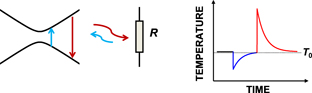
Next we discuss the calorimetric measurement of the energy deposited on the resistor. The electronic system of the resistor forms the environment that is then coupled to a super-bath formed, e.g. by phonons to which these electrons couple by standard electron–phonon coupling. This leads to the following sequence once an energy quantum ΔE is emitted/absorbed by the two-level system due to ∓ transitions, see figure 3. We assume the standard hot-electron regime [34, 35]. (i) The temperature T of the resistor (electrons) changes abruptly by  at the moment of the photon exchange; here
  is the heat capacity of the electron gas in the resistor. (ii) The electronic temperature of the resistor starts to relax back toward the equilibrium T0 ≡ (kBβ)−1 at the rate governed by the thermal conductance G that is determined, e.g. by electron–phonon coupling. (iii) New energy pulses may occur during the evolution. In this evolution the deposited energy (heat) to the bath can be obtained generally from
  , where ΔT = T − T0. Note that the pulses can have either + or − sign, i.e. the resistor may cool as well. In the considered example,
  , where ΔEi is the magnitude of heat released in the ith absorption/emission event, and ti are the time instants of these events. Note that unlike in the analysis leading to (1) and (2), we allow here different values for ΔEi for transitions occurring along the driven trajectory. Integrating the equation for
  for the situation where the system is in thermal equilibrium in the beginning and at the end, i.e. T(0) = T(∞) = T0, and assuming small temperature rise in the pulses, we have for the heat in each realization

To make full use of (17), the following practical issues need to be taken care of [35]. The thermometer is first calibrated against the bath temperature under the equilibrium conditions (without applying the driving field), or one uses a primary thermometer that serves without calibration. The only remaining calibration is then the determination of G: this can be obtained by applying a known constant power P to the calorimeter, and measuring the temperature rise δT of the electrons in the thermometer, since G = P/δT.
Figure 3. Schematic presentation of the calorimetric measurement. The resistor in the middle emits (absorbs) heat to (from) the two-level system on the left upon excitation (relaxation) shown by blue (red). The corresponding heat pulses, i.e. temperature of the electrons in the resistor versus time, are shown on the right with the same color conventions. We assume that the electrons are in the so-called hot-electron regime, where the internal (electron–electron) relaxation is faster than other time scales in the problem.
Download figure:
Standard image High-resolution image
Before turning to the detailed practical realization and numbers, one further consideration is in order. Namely, biasing the gate capacitor in the ramp that we consider leads to a current that dissipates Joule power ΔEd in the resistor R. This dissipation can be estimated by elementary circuit analysis with the result ΔEd = e2R/τ. For typical values of τ and R, for instance those in figure 2, this energy is at most of order 0.01 EC. Since EC is the scale of work performed, the Joule heating produces only a small error in the calorimetric measurement, even if no precautions are taken.
We analyze next the feasibility of measuring calorimetrically the distribution of quantum work in a superconducting two-level system considered. The most straightforward realization would involve a small lithographic metal resistor, ∼ (0.1 μm)3, on the chip [36]. The electronic heat capacity at T0 = 100 mK temperature is  , yielding a jump in temperature of
  upon absorbing the relaxation heat at the end of the ramp, assuming a realistic EC/kB = 3 K. This is a sizable change of temperature (3%) which can be detected over a relatively long time of order 10−4 s that is determined by the equilibration of the resistor back to its initial temperature via electron–phonon coupling. The large sensitivity of the calorimeter is naturally due to the standard T0/TF ∼ 10−6 suppression of the heat capacity of the electron gas with Fermi temperature TF ∼ 105 K. If needed, longer relaxation times can be obtained by, for instance, suspending the resistor on a silicon nitride membrane [37], which would make the detection even easier. A tunnel probe, in form of a superconducting lead connected to the resistor, i.e. a superconductor–insulator–normal metal (SIN) junction, measured by RF reflection or transmission techniques [38], is fully compatible with the requirements of the presented calorimetric detection of heat.
In the current work we considered only one quantum system (CPB) in a specific (incoherent) regime as an illustration of the calorimetric method. Yet the same detection method can be applied to a large class of systems, where the validity of the fluctuation relations is not necessarily obvious unlike in the current example. First of all, the CPB in a weak dissipation regime is a qubit that obeys nearly coherent evolution and to be precise, an analysis respecting energies down to EJ ≪ EC is needed. The calorimetric measurement applies, with equal conditions, also to this regime, but here the distribution of dissipation would have more structure at low energies and the theoretical assessment of the fluctuation relations would be less obvious. Secondly, the calorimetry can be applied to any system, where (i) the coupling between the quantum system and the calorimeter is the dominant energy relaxation channel, and where (ii) the sensitivity and the bandwidth of the thermometer are sufficiently high for observing the exchange of photons. These conditions are valid for mesoscopic electronic circuits quite generally. Instead of a CPB, one may envision other kinds of superconducting qubits [39], such as flux qubits (SQUIDs), where the coupling to the calorimeter can be provided inductively. Moreover, (semiconducting) quantum dot circuits [40] can be coupled capacitively to the dissipative calorimeter, similarly to what was presented for CPB here. This method can measure dissipation in many-body systems as well, as long as the systems can be coupled to a calorimeter. This way the number of possible applications of the method would be further increased [41–43].
In conclusion, the calorimetric measurement yields a direct determination of quantum work and quantum fluctuation relations. It can be used to analyze theoretically and experimentally the work and its distribution in a quantum system.
Acknowledgments
We thank J Ankerhold, S Gasparinetti, D Golubev, F Hekking, M Möttönen, J Santos and P Wollfarth for discussions. The work was supported partially by LTQ (project no. 250280) CoE grant, by the Academy of Finland through its Centres of Excellence Program (project no. 251748) and the European Community's Seventh Framework Programme under grant agreements no. 238345 (GEOMDISS) and no. 308850 (INFERNOS).