


Abstract
We calculate the correction to the electronic density of states in a disordered ferromagnetic metal induced by spin-wave mediated interaction between the electrons. Our calculation is valid for the case that the exchange splitting Δ in the ferromagnet is much smaller than the Fermi energy, but we make no assumption on the relative magnitude of Δ and the elastic electronic scattering time τel. In the 'clean limit' Δτel/ℏ ≫ 1 we find a correction with a Td/2 temperature dependence, where d is the effective dimensionality of the ferromagnet. In the 'dirty limit' Δτel/ℏ ≪ 1, the density-of-states correction is a non-monotonous function of energy and temperature.

Content from this work may be used under the terms of the Creative Commons Attribution 3.0 licence. Any further distribution of this work must maintain attribution to the author(s) and the title of the work, journal citation and DOI.
1. Introduction
Whereas quantum corrections to the electronic properties of normal metals have been studied theoretically and experimentally for almost half a century [1–4], the electronic properties of ferromagnetic metals only attracted attention at a later stage, mainly triggered by the emergence of the field of spintronics [5]. Conceptually simple devices, such as a ferromagnet–insulator–ferromagnet junction, were found to exhibit spectacular magnetoresistive effects [6, 7]. Ferromagnet–superconductor junctions display a wide range of interesting phenomena, including inhomogeneous induced superconductivity [8], polarization-dependent Andreev scattering [9] and induced triplet superconductivity [10], all stemming from the different spin-orderings in ferromagnets and (s-wave) superconductors. In the context of these fairly recent discoveries, a detailed understanding of the electronic properties of disordered ferromagnets is quintessential.
Although the two key elements determining quantum corrections in normal metals, disorder and Coulomb interactions, also play a role in ferromagnets, the existence of magnetic order in ferromagnets adds additional complexity. The very presence of the magnetic order, but also its quantum and thermal fluctuations, modify quantum corrections to electronic properties in an essential way. For example, spin–orbit interaction couples the orbital motion of electrons to the exchange field of the magnet, causing an anomalously strong dependence of the conductivity on magnetization direction [11, 12]. Also electronic scattering from spatial or temporal inhomogeneities of the magnetization in space and time, such as domain walls and spin waves, can lead to dephasing [13, 14] and it can qualitatively affect the metallic resistivity [15–17].
In this paper we address the tunneling density of states, which is a key property in devices in which metallic and insulating layers alternate. For a normal metal, the interplay of disorder and Coulomb interaction effects causes the tunneling density of states to deviate from the thermodynamic density of states for low temperatures and excitation energies [2, 18–20]. In three dimensions, the temperature dependence of the correction to the density of states follows a square-root power law. While it is clear that for a weakly disordered ferromagnet the same effects modify electronic density of states, in a ferromagnet fluctuations of the magnetic order may cause an additional correction to the density of states.
About a decade ago, a series of experiments on ferromagnetic tunnel junctions [21] revealed a T3/2 power law up to room temperature of the tunnel resistance and magnetoresistance of the junctions [22, 23]. MacDonald et al [24] linked this observation to a reduction in the average (surface) polarization of the magnets, caused by thermally excited spin waves, which is indeed known to have a T3/2 dependence [25]. Essentially, the mechanism of MacDonald et al [24] is that thermal fluctuations of the magnetization, which in [24] is assumed to be fully carried by the conduction electrons, smear the difference between majority and minority electron densities of states.
In this paper, we revisit the question of a spin-wave-mediated correction to the density of states. We take the viewpoint that the emission and absorption of spin waves leads to an effective interaction between the electrons (in the same way as that the emission and absorption of phonons leads to an effective electronic interaction in the theory of superconductivity), and consider the resulting correction to the density of states for a disordered ferromagnet, analogous to the Coulomb-interaction induced correction to the density of states of a normal metal. Remarkably, in the most relevant parameter range we find the same T3/2 dependence of the correction to the density of states as in [24], although our calculation does not rely on different (bare) densities of states for majority and minority electrons. We note that quantum corrections to the conductivity and the dephasing rate that arise from an effective spin- wave-mediated electron–electron interaction have been considered previously by various authors [17, 26, 27]. However, we are not aware of a calculation of the effect on the tunneling density of states.
Our calculations are performed using diagrammatic perturbation theory. A key condition for applicability of this approach is that the exchange splitting between majority and minority spins Δ be much smaller than the Fermi energy EF. We note that this condition is not met for strong ferromagnets, such as Fe or Ni, for which Δ and EF differ less than one order of magnitude. Nevertheless, we point out that our calculation provides a controlled theoretical estimation of the effect of the effective spin-wave-mediated interaction, as it identifies temperature and energy dependences of the density of states that are unrelated to a difference in the bare densities of majority and minority electrons. Our calculations do not rely on the diffusion approximation, so that Δ may be large or small in comparison to the elastic scattering rate ℏ/τel. This is important, because most realistic ferromagnets are in the 'clean limit', in which Δτel/ℏ ≳ 1.
The precise microscopic model we consider is described in section 2. The calculation of the leading correction to the density of states using diagrammatic perturbation theory is given in section 3, followed in section 4 by a discussion of the result in the limits of a clean and a dirty ferromagnet (Δ large or small in comparison to ℏ/τel, respectively). Our main result is a clean-limit density-of-states correction proportional to Td/2 or | |d/2 in an effectively d-dimensional ferromagnet, where is the excitation energy (measured with respect to the Fermi energy). In the dirty limit we find a non-monotonous energy and temperature dependence. We conclude with a comparison to the correction to the density of states from Coulomb interactions in section 5.
2. Model
To describe the conduction electrons in the disordered ferromagnet and their interaction with fluctuations of the magnetization of the d-band electrons, we use the same model as employed in [14]. An identical model description has been used for ferromagnetic metals in which the magnetism resides with itinerant electrons only [24]. In this model, the electrons are described with the effective single-particle Hamiltonian

where the first term represents the kinetic energy, μ is the chemical potential, V (r) is the impurity potential and the last term describes the exchange interaction between the conduction electrons and the d-band electron spins. In the exchange term, J is the exchange constant and ℏs(r) is the spin density of the d-electrons.
We choose the z-axis such that it points in the direction of the mean d-band magnetization, and we write


The mean magnetization gives rise to an effective exchange splitting and the coupling to the fluctuations around this mean value are described by Hsd,fluc.4 To linear order in the fluctuations we can focus on the transverse components sx,y(r,t),


where we use the notation s± = sx ± isy.
Dynamical processes involving the absorption and excitation of a d-band spin wave are characterized by the transverse spin susceptibility

where Θ(τ) = 1 for τ > 0 and Θ(τ) = 0 otherwise is the Heaviside step function. The susceptibility χR−+(r,τ) describes the response of the d-electron spin density to an applied magnetic field. Its Fourier transform χR−+(q,ω) is conveniently expressed in terms of the spin wave frequencies ωswq = ωsw−q [26, 28],


where η is a positive infinitesimal. The susceptibility for opposite spin orientations reads

The spin wave frequencies ωswq are determined by interactions and anisotropy factors not taken into account in the conduction electron Hamiltonian (1). Following [17, 27] we assume the phenomenological isotropic spin-wave dispersion relation

Here Dsw is the spin wave stiffness, usually of the order ℏDsw ∼ Δ/k2F. The constant Δsw gives the spin wave gap, which can be due to, e.g. an externally applied magnetic field in the z-direction or by the magnetocrystalline anisotropy of the material. In the former case, one has Δsw = gμBB, where is the external magnetic field corrected for the demagnetizing field of the device, ξ being a numerical constant determined by the shape of the ferromagnet [29]. In the latter case , where K is the energy density characterizing the anisotropy.


3. Perturbative calculation
The emission and absorption of spin waves gives rise to an effective interaction between the electrons. For nonzero spin-wave gap this interaction is short-range, and its effect on the electronic density of states of a disordered ferromagnet can be calculated via diagrammatic perturbation theory. In order to apply the diagrammatic perturbation theory it is necessary that all relevant energy scales be small in comparison to the Fermi energy EF. In the present case, this means that the exchange splitting Δ and the elastic scattering rate ℏ/τel must be small in comparison to EF. No assumptions need to be made with regard to the relative magnitude of Δ and ℏ/τel. The condition Δ ≪ EF is not met (as a strong inequality) for the elemental ferromagnets, which means that for those materials our results should be seen as order-of-magnitude estimates.
The same condition Δ ≪ EF implies that, without the spin-wave-mediated correction, majority and minority electrons have the same density of states ν at the Fermi level, the same Fermi velocity vF, and the same elastic scattering time τel. (As shown below, we will find that for the clean limit Δτel/ℏ ≫ 1 the corrections do not depend on τel, rendering it thus unnecessary to keep track of two different scattering times.) Consistent with these expectations, for the impurity potential we take a Gaussian white noise distribution

where ν is the conduction electron density of states (per spin direction) and τel the elastic mean free time.
In diagrammatic perturbation theory, the leading correction to the density of states νσ for electrons with spin σ = ± 1 is given by the 'Fock' diagram shown in figure 1(a). The 'Hartree' correction is absent because of the spin-flip nature of the sd interaction term. Expressing this correction in terms of the exact retarded and advanced Green functions GRσ(r,r',) and GAσ(r,r',) of the conduction electrons, and using the identity

one finds

where is the sample volume. In order to ensure convergence of the integration at large energies ζ, we later subtract the zero-energy zero-temperature correction δνσ(0,0) from the expression for δνσ(,T) shown above.


Figure 1. (a) Diagram representing the leading-order correction to the density of states. Solid lines denote the conduction electron Green functions, the wiggly line represents the spin-wave propagator χ−σ,σ. (b) Dressed interaction vertex for a disordered ferromagnet. The dashed line with the cross represents correlated elastic impurity scattering.
Download figure:
Standard image High-resolution imageIt remains to average the products of the electronic Green functions over the disorder. For the two contributions to δν(,T) that contain a product of two retarded Green functions, we may replace the product of the Green functions by the product of the ensemble-averaged Green functions 〈GR−σ(r2,r1,)〉 = 〈GR−σ(r2 − r1,)〉. Changing to the Fourier representation, the density of states correction can be expressed as a summation over spin-wave wave vectors q. One then quickly finds that these two contributions vanish, as long as the relevant wave numbers q ≪ kF.
Such a procedure cannot be applied to the term that has a product of a retarded Green function and an advanced Green function. Here impurity scattering renormalizes the two vertices for the electron–spin-wave interaction, see figure 1(b). The result is most conveniently expressed as

where the bare structure factor Πσ,−σ(q,,') is expressed in the disorder-averaged Green functions as

Using the explicit expressions for the disorder-averaged Green functions,

with k = ℏ2k2/2m − μ, one finds that, as long as , ' ≪ EF, the structure factor depends on the energy difference − ' only,

Substituting equation (6) for the transverse spin susceptibility, one arrives at the final expression

This expression, with equation (14) for Πσ,−σ, presents the most general result obtainable within the perturbative approach and is the starting point for our further analysis. It does not rely on the diffusion approximation, i.e. on the smallness of Δ, ℏωswq or vFq with respect to ℏ/τel, and instead only assumes smallness with respect to EF.
We note here that it follows from equation (15) that

However, there is no symmetry relation relating the density-of-states corrections δν↑ and δν↓ at equal energies, and in general δν↑(,T) will be different from δν↓(,T) if ≠ 0. In our model, no difference between ν↑ and ν↓ appears at zero energy. Because of the symmetry (16), we can focus on one particular spin direction, say spin up, without loss of generality, and the results for the other spin direction as well as the total correction δν↑ + δν↓ to the density of states simply follow from the symmetry relation (16).
4. Asymptotic behavior of the correction
Inserting the spin wave dispersion relation (8)—or, if desired, a more detailed dispersion including shape-dependent terms and various anisotropies [29]—equation (15) can be numerically integrated to give the energy and temperature dependence of the density-of-states correction for general values of the parameters. The contributions from the poles can be regularized by adding a small positive imaginary part to the integration variable ζ, which preserves the causal dependences of equation (15). (Results will not depend on the value of the infinitesimal added.)
For the limiting case of a clean ferromagnet, Δτel/ℏ ≫ 1, it is possible to simplify equation (15) considerably and to arrive at analytic results. Below we will present the resulting corrections to the density of states in this clean limit for three-, two-, and one-dimensional samples, and we will also present numerical results for the opposite dirty limit where Δτel/ℏ ≪ 1.
4.1. Clean limit
We first describe the case of a clean ferromagnet, for which the inequality Δτel/ℏ ≫ 1 holds. If, in addition, we also assume that Δ ≫ ℏqvF for all q which contribute significantly to the sum in (15), the expression for the spin-wave correction to the density of states can be significantly simplified. Below we will show that this restriction is equivalent to assuming that Δ ≫ E2/3Fmax{T1/3,||1/3}, which is not in contradiction with Δ ≪ EF but limits the validity of our approach to temperatures and energies T,|| ≪ Δ3/E2F.
Using the inequalities Δτel/ℏ ≫ 1 and Δ ≫ ℏqvF, one can expand (15) for large Δτel/ℏ, yielding to leading order in ℏ/Δτel

This result does not depend on τel, which implies that all spin wave mediated electron–electron interactions are short-range and take place on a length scale much smaller than the elastic mean free path lel = vFτ. Furthermore, we note that the apparent divergence of equation (17) from the contribution from large wave vectors q → ∞ is canceled if one calculates the difference with the zero-temperature zero-energy correction to the density of states,

which gives

where nF() is the Fermi function. Indeed, after subtracting δν↑(0,0), all contributions coming from spin waves with an energy ℏωswq ≳ max{T,||} are exponentially suppressed. Therefore, from the dispersion relation (8) we see that the largest momenta which we have to take into account are of the order

In order to satisfy Δ ≫ ℏqvF for all q in the summation, we thus find the constraint Δ ≫ ℏqmaxvF. Using that typically ℏDsw ∼ Δ/k2F we recover the constraint anticipated above.
For ferromagnetic samples with large enough dimensions the summation over q can be replaced by an integral which can be explicitly evaluated. If all three dimensions are much larger than q−1max, we can treat the sample as three-dimensional and convert the sum over q to an integral over spherical coordinates. If one or two of the dimensions are small enough, a ≪ q−1max (but still a ≫ lel), the effective dimensionality for the spin waves becomes lower, and the integral over q becomes two- or one-dimensional as well. The constraint a ≪ q−1max corresponds to the regime of low temperatures, where T ≪ ℏDsw/a2. For example, for a thin Fe sheet or wire with thickness/diameter a = 10 nm, we find that a lower dimensional treatment is justified only if T ≪ 800 mK using typical parameters for iron [30, 31]. The restrictions on the temperature are however not always that severe. For instance, for the thin Gd films studied in [17] and using their estimates for the material parameters, we find that the samples are effectively two-dimensional up to temperatures of a few times 10 K. We note here that we take the system size in all dimensions to be larger than the electronic elastic scattering length, so that electronic transport is diffusive in all directions.
In keeping with the effective d-dimensional description, we introduce d-dimensional exchange constants and magnetization densities, by replacing J → J/a3−d and . Hence, J and now have respectively dimensions of energy times volume, area or length and polarization per volume, area or length. We then find


where is the polylogarithm. The polylogarithm has the asymptotic behavior


while Lid/2(− 1) is a weakly d-dependent number of order unity [Li1/2(− 1) ≈ −0.605, Li1(− 1) ≈ −0.693 and Li3/2(− 1) ≈ −0.765].
The energy and temperature dependence of δν*σ and of the total density-of-states correction δν* = δν*↑ + δν*↓ is shown in figure 2 for the case d = 3. The top panel shows the -dependence for three representative values of the temperature (larger, equal to and smaller than the spin-wave gap Δsw). The bottom panel shows the temperature dependence at zero energy.

Figure 2. (top) The total density-of-states correction δν* = δν*↑ + δν*↓ as a function of /T for three different ratios Δsw/T of the spin wave gap Δsw and the temperature, for a three-dimensional sample. The relative density-of-states correction is given in units of . For Δsw = 0 (no spin-wave gap) the corrections for spin-up and spin-down electrons are shown separately (dashed lines). (bottom) The temperature dependence of δν*(0,T)/ν at zero energy, as a function of the ratio T/Δsw of temperature and spin-wave gap. The relative density-of-states correction is given in units of .


Download figure:
Standard image High-resolution imageExpanding equation (20) around = 0 one finds that for small energies, the correction to the total density of states is quadratic in /T,

where we introduced A1 = −2Lid/2(− e−Δsw/T ) and A2 = −Li(d−4)/2(− e−Δsw/T ). Both constants reduce to numbers of order unity when the temperature is much larger than the spin-wave gap.
In the limit of (i) very small temperatures or (ii) very far away from the Fermi energy, where T ≪ |Δsw ± |, we can use the asymptotic properties of the polylogarithm to find

if || > Δsw, whereas δν(,0) = δν(0,0) if || < Δsw. At low temperatures, the correction to the density of states ceases to be energy dependent for energies which lie closer to the Fermi energy than the spin wave gap energy Δsw. Indeed, at zero temperature the only relevant energy-dependent process is the excitation of spin waves by minority spin electrons or majority spin holes with an energy of at least the spin wave gap away from the Fermi energy.
The temperature dependence of the correction to the density of states also follows from equation (20) and the asymptotic dependences of the polylogarithm. In particular, at the Fermi energy = 0 one finds that δν* is proportional to Td/2 for temperatures T much larger than the spin-wave gap. The temperature dependence δν*σ(0,T)∝T3/2 for d = 3 is the same as the one found in [24] from a different microscopic mechanism. An important difference with [24] is that for the mechanism we consider δν↑(0,T) = δν↓(0,T), whereas δν↑(0,T) = −δν↓(0,T) in [24].
4.2. Dirty limit
We now consider the regime Δτel/ℏ ≪ 1 of a dirty ferromagnet. We make the additional assumption that the wave number and energies of all thermal spin waves involved are low enough that qvFτel, ωswτel ≪ 1. This additional assumption allows us to use the diffusion approximation and expand in small Δτel/ℏ, as well as qvFτel and ωswτel, which considerably simplifies equation (15).
Although our additional assumption qvFτel, ωswτel ≪ 1 is commonly used in the literature [17, 26, 27], it poses a rather severe (but not impossible5) restriction on the temperature T and energy : . (The restriction is 'severe' because ℏ/EFτel is the small parameter of the perturbation theory.) The origin of the smallness of allowed temperatures and energies is the large mismatch of the spin wave stiffness and the electronic diffusion constant in the dirty limit, D/Dsw ∼ ℏ(kFlel)2/(Δτel) ≫ 1.

In the diffusion approximation, the quantity 1/[1 − Πσ,−σ(q,ζ)] appearing in the expression (15) for the density-of-states correction becomes equal to the diffusion propagator

where D = v2Fτel/d is the diffusion constant for the conduction electrons in d effective dimensions. For the correction to the density of states this leads to

Although equation (24) can be further evaluated, e.g. in the limit of zero temperature, the resulting expressions are too complex to be insightful, and we therefore prefer a numerical evaluation of the double integral in equation (24) in a few representative limits. Results are shown in figures 3 and 4. In both cases we have set the ratio Dsw/D = 10−3, consistent with the large mismatch between these two constants mentioned above.

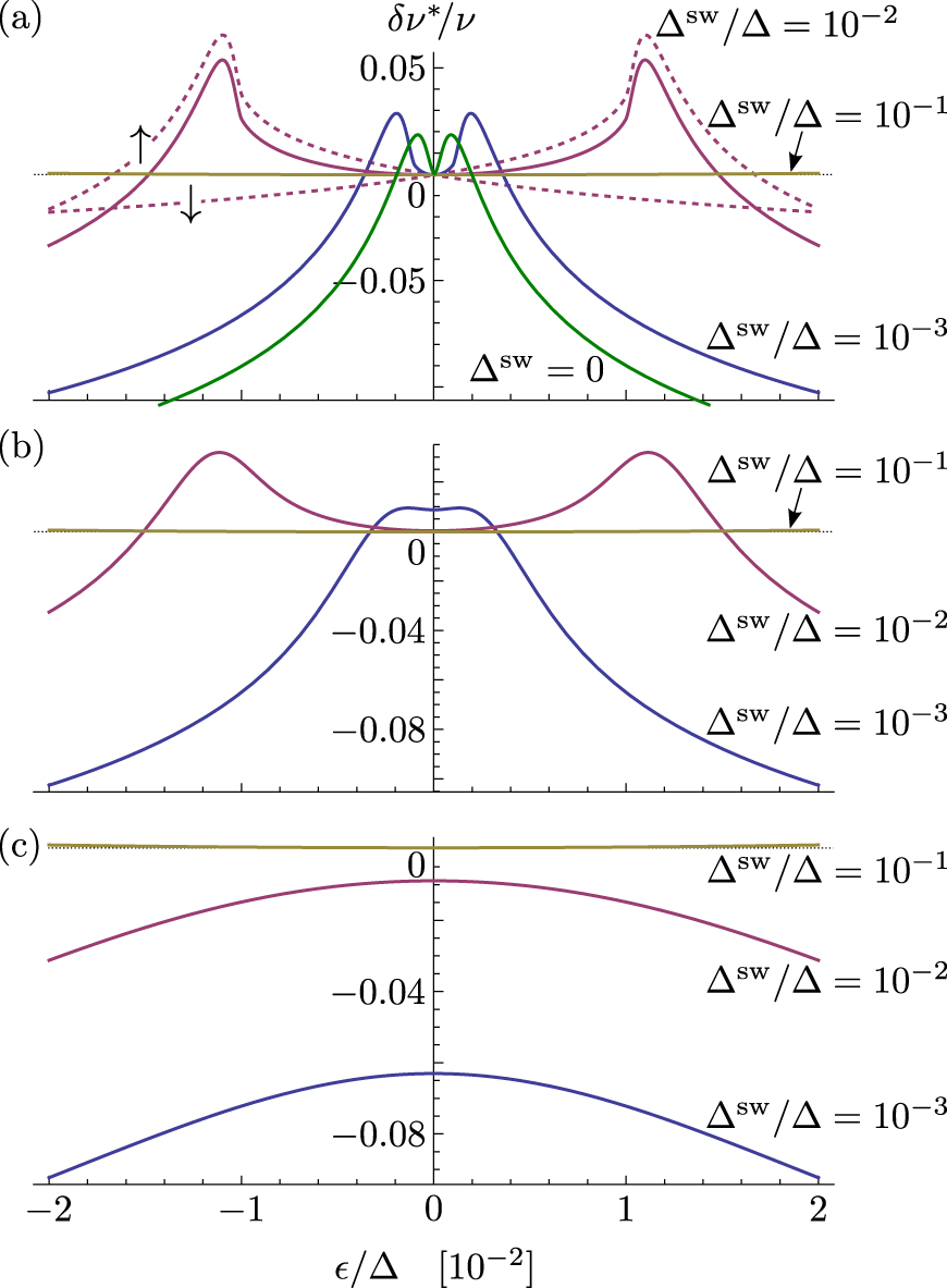
Figure 3. Spin-wave induced correction to the density of states for a three-dimensional dirty ferromagnet. We show the correction close to the Fermi energy for three different spin wave gaps Δsw as indicated in the figure. The temperature was set to (a) T = 0, (b) T = 10−3Δ and (c) T = 10−2Δ. The resulting relative correction δν*(,T)/ν is plotted in units of . We have set Dsw/D = 10−3 in all cases. In (a) we show the corrections at Δsw/Δ = 10−2 for majority electrons (↑) and minority electrons (↓) separately (dashed lines), showing that the peak at negative (positive) energy stems from the correction to the majority (minority) density of states.

Download figure:
Standard image High-resolution image
Figure 4. Correction to the density of states for a three-dimensional dirty ferromagnet at zero energy as a function of temperature. Curves are shown for three different spin wave gaps Δsw, as indicated in the figure. The relative correction δν*(0,T)/ν is again plotted in units of . We have set Dsw/D = 10−3 throughout.

Download figure:
Standard image High-resolution imageIn figure 3 we show the correction δν*(,T) for different ratios of the spin-wave gap Δsw and the exchange splitting Δ and for different values of the temperature. The figure shows a remarkable non-monotonous dependence on the excitation energy . This dependence can be most easily understood for the case of zero spin-wave gap and zero temperature (Δsw = 0, green line in figure 3(a)). At the smallest energies, || ≪ (Dsw/D)Δ, we find that the maximal wave number contributing to the sum in equation (24) is . This implies that for all relevant spin-wave energies we have ℏDq2 ≪ Δ leading to Dσ,−σ(q,ζ) ≈ ℏi/Δτel. This means that a typical spin-wave excited electron–hole pair still dephases before it diffuses significantly through the sample, yielding a situation similar to that of the clean ferromagnet treated above. Indeed, if we take ζ ≪ Δ and ℏDq2 ≪ Δ, then equation (24) reduces exactly to the clean result (19). The correction at small energies then has the same (positive) sign as found before. On the other hand, at large excitation energies || ≫ (Dsw/D)Δ, we can simplify (24) using that for most wave numbers q contributing to the summation we have Dσ,−σ(q,ζ) ≈ 1/Dq2τel, leading to a different sign in (24). Indeed, this is a truly diffusive limit, in which the excited electron–hole pairs can diffuse over long distances. The effective spin wave mediated electron–electron interaction Usw(q,iωn) = J2[χ−+(q,iωn) + χ+−(q,iωn)] < 0 is of an attractive nature, for which in the diffusive limit the exchange correction is known to yield a correction negative for increasing energy [2]. With a finite spin-wave gap Δsw the resulting peaks are shifted by Δsw, as seen in figure 3(a)). At higher temperatures, as shown in figures 3(b) and (c), the peaks are smeared out and the correction tends to be a smooth peak centered at the Fermi energy.

In figure 4 we show the temperature dependence of the correction to the DOS at the Fermi level = 0, using temperatures small enough that the condition T,|| ≪ Δℏ2/(EFτel)2 can be satisfied. The non-monotonous temperature dependence has the same origin as the non-monotonous energy dependence of figure 3. When the temperature is larger than the spin wave gap, T ≳ Δsw, the thermal broadening of the double peak structure around the Fermi level becomes strong enough to reduce δν(0,T) below the reference value δν(0,0), which results in a change of sign.
5. Conclusion
For the spin wave induced correction to the density of states we find qualitatively different results depending on whether Δτel/ℏ is small or large. For the clean limit Δτel/ℏ ≫ 1, which is the most realistic situation, we derived an analytical expression for the density-of-states correction δν(,T) for one-, two-, and three-dimensional samples. At zero excitation energy (measured with respect to the Fermi energy) in a d-dimensional sample the correction has a power-law temperature dependence δν*∝Td/2 for temperatures larger than the spin wave gap Δsw. At T = 0 and away from the Fermi level, the energy dependence of the correction also follows a power-law, δν*∝(|| − Δsw)d/2 for energies larger than Δsw. In the dirty limit Δτel/ℏ ≪ 1 we found that the correction to the density of states has a non-monotonous dependence on energy and temperature, with a peak for temperatures or energies near the spin-wave gap Δsw.
Relevant questions to address are how large the correction is in comparison with the correction resulting from electron–electron (Coulomb) interactions in the ferromagnet and how it compares to the mechanism of [24]. For the first question we restrict ourselves to the experimentally most relevant clean limit Δτel/ℏ ≫ 1. In three dimensions the correction due to electron–electron interactions is [2]

for very low temperatures and

at the Fermi level. The corresponding spin-wave-induced corrections found here have a power-law dependence of (neglecting the spin-wave gap Δsw for simplicity). This means that at small energies and temperatures the correction due to electron–electron interactions dominates, and that there are minimum energy and temperature scales min and Tmin above which the spin wave induced correction can become the dominant one. A straightforward comparison of the two corrections yields


Since EFτel/ℏ is the large parameter of the perturbation theory, this is well within the validity range of the diagrammatic perturbation theory. Using typical parameters for Fe [30, 31], we estimate this crossover scale as ∼ 1 K. We thus expect the temperature dependence of the density-of-states correction to be given by a T3/2 power law for temperatures above Tmin.
The density-of-states correction of [24] is, again to second order in the exchange coupling J

where nB is the Bose–Einstein distribution function and ν↑ and ν↓ are the unperturbed densities of states for majority and minority electrons, respectively. This expression is similar to our result (19) for the clean limit, which has the factor νσ − ν−σ replaced by ν and the Bose–Einstein factor nB(ℏωswq) replaced by the Fermi factor nF( + ℏωswq). Since typically nB ≫ nF, we conclude that the magnitude of the correction of [24] is larger than the correction calculated here in the case of a strong ferromagnet, for which |ν↑ − ν↓| ∼ ν. Distinguishing the two corrections should still be possible, because of the singular dependence of the correction calculated here on the excitation energy . (No singular -dependence is reported in [24].)
Acknowledgments
We gratefully acknowledge helpful discussions with Georg Schwiete and Martin Schneider. This work was supported by the Alexander von Humboldt Foundation in the framework of the Alexander von Humboldt Professorship program, endowed by the Federal Ministry of Education and Research.
Footnotes
- 4
As explained in [14], this exchange splitting Δ can differ from if exchange interactions between conduction electrons are taken into account. We will thus not make use of the relation , but keep Δ as an independent parameter instead.
- 5
For a dirty ferromagnet with EF ∼ eV and having, e.g., EFτ/ℏ ∼ 20 (which then corresponds to an electronic elastic scattering time of the order of 10−14–10−15 s), we find the two constraints mentioned above to be Δ ≪ 1000 K and T,|
| ≪ Δ/400. This means that, although on the edge of the regime of validity, the diffusive approximation could work in certain cases for energies and temperatures up to ∼1 K.

