


Abstract
Coherent multidimensional spectroscopy allows us to inspect the energies and the coupling of quantum systems. Coupled quantum systems—such as a coupled semiconductor quantum dot or pigments in photosynthesis—form delocalized exciton and two-exciton states. A technique is presented to decompose these delocalized wave functions into the basis of individual quantum emitters. This quantum state tomography protocol is illustrated for three coupled InAs quantum dots. To achieve the decomposition of the wavefunction, we combine the double-quantum-coherence spectroscopy with spatiotemporal control, which allows us to localize optical excitations at a specific quantum dot. Recently, a protocol was proposed for single exciton states (Richter et al 2012 Phys. Rev. B 86 085308). In this paper, we extend the method presented by Richter et al with respect to: the reconstruction of two-exciton states, a detailed analysis process of reconstruction and the effect of filtering to enhance the quality of the reconstructed wave function.
Export citation and abstract BibTeX RIS

Content from this work may be used under the terms of the Creative Commons Attribution-NonCommercial-ShareAlike 3.0 licence. Any further distribution of this work must maintain attribution to the author(s) and the title of the work, journal citation and DOI.
1. Introduction
Complex (hybrid) nanostructures are often formed by combining different individual nanostructures such as metal nanoparticles, semiconductor quantum dots (QDs), pigments embedded in proteins, such as in light harvesting complexes and J-aggregates [1–10]. Couplings (such as Coulomb couplings) between the individual emitters lead to the formation of new quantum states delocalized over the individual nanostructure.
Far-field optical experiments cannot resolve the internal structure of the delocalized states since the applied electric field is spatially constant on the spatial dimension of the nanostructure, which is much smaller than the excitation wavelength. Therefore only the collective formed delocalized exciton states are accessible in far-field spectroscopy. For disentangling the individual contributions to delocalized states, a form of near-field spectroscopy is needed. There have recently been many experiments demonstrating that spatiotemporal control of optical excitations can be achieved by combining pulse shaping techniques with nanoplasmonics [11–13]. There are also even experiments that demonstrate how nanometer spatial resolution and two-dimensional (2D) spectroscopy can be combined [14]. Other techniques for spatiotemporal control include near-field techniques such as (metalized) fiber tips [1, 12, 15–17] or nano-antennas [18–23].
While nonlinear 1D spectroscopy provides the energy and spectral shape of exciting coupled quantum systems, coherent multidimensional spectroscopy allows to also investigate the couplings between the states [24, 25]. Multidimensional spectroscopy gives a deeper insight into the underlying microscopic processes.
Combining coherent multidimensional spectroscopy with spatiotemporal control of exciting pulses promises to reveal more information about the system than 2D spectroscopy or localization alone [14]. We extend the reconstruction method for delocalized single excitons presented in [26] from single excitons to two excitons.
In section 2, double-quantum coherence 2D spectroscopy is described [24]. After presenting the double-quantum coherent spectroscopy [24, 27, 28], the treatment of the coupling of the QDs is described. Then, 2D spectra and their signal are discussed. In section 3, the focus is on localized spectroscopy: firstly, examples of spatiotemporal control are explained; next, the description of the spectra from section 2 is generalized to localized excitation. Then, the method of reconstructing the exciton as well as the two-exciton wave function coefficients is presented in detail. Finally, the filtering method—introduced in more detail in [26]—is applied to improve the quality of reconstruction. Here, we discuss also quantitatively the influence of filtering on the reconstruction. The paper is aimed at an extension of the methods from [26] towards determination of two-exciton wave functions.
2. Two-dimensional (2D) spectroscopy
1D nonlinear spectroscopy techniques such as pump–probe or four-wave mixing experiments allow us to investigate the time evolution of quantum states and transition energy of the excited states.
Coherent multidimensional spectroscopy [12, 24, 27–37] provides new insights into the structure of several complex molecular and nanoscale systems such as photosynthetic aggregates or semiconductors [1, 2, 7, 24, 38]. Recently, even the application of coherent spectroscopy to GaAs natural QDs was reported [39–41]. Coherent spectroscopy uses multiple excitation pulses together with direction selection or phase cycling to control the quantum pathways of excitation. The delay times between the pulses are varied giving a signal dependent on multiple dimensions.
2.1. Setup and simulation
In four-wave mixing experiments the sample is excited by a sequence of three pulse envelopes

separated by variable time delays t1, t2 and t3 with different phases φ1, φ2 and φ3 and laser frequency ωl (illustrated in figure 1(a)). Since we treat only a single nanostructure, a dissection of quantum pathways using the direction of the incoming fields is not possible. Therefore, a phase cycling technique is applied. Here, the simulated experiment is carried out several times with different phase contributions φ1, φ2 and φ3. This allows us to extract a specific signal, described by the linear combination φS = lφ1 + mφ2 + nφ3 of the phases using postprocessing algorithms (where l, n and m are integers). To extract a certain polarization Pl,m,n from the detected polarization  , the experiment is repeated for sufficient phase combinations [42] (determined by the matrix ei(lφ1+mφ2+nφ3)), so that the polarization Pl,m,n can be extracted by inverting the matrix ei(lφ1+mφ2+nφ3).

Figure 1. In (a), the pulse sequence of the double-quantum-coherence signal is shown. Part (b) illustrates the delocalized states of the coupled QD system.
Download figure:
Standard imageIn this paper, we focus on double-quantum-coherence spectroscopy (DQCS), where the extracted phase combination is φIII = φ1 + φ2 − φ3. Two Liouville pathways contribute to this signal for a three-band system as depicted in figure 1(b). The pathways are shown in figure 2, presented by double-sided Feynman diagrams [29]: in both quantum pathways, the first pulse creates a coherence between the ground state and a single exciton, and the second pulse creates a coherence between a two-exciton and the ground state. The third pulse creates in pathway (i) a single exciton to ground state coherence, whereas in pathway (ii) a two-exciton to single exciton coherence is created. The fourth pulse depicted in figure 1(a) is the local oscillator for heterodyne detection [24]. This allows a detection of the signal phase.

Figure 2. Double-sided Feynman diagram that shows two possible pathways for the DQCS.
Download figure:
Standard image2.2. Coupled quantum dots
In the following, QDs—as an example of a system of coupled nanostructures—are examined in the 2D spectroscopy experiment. We will demonstrate that the DQCS can reveal the energy of single and two-exciton states of the coupled QDs [24, 43].
As a model system, we examine n = 3 coupled QDs that are spatially close enough to couple via Förster coupling but spatially separated enough to have no wave function overlap. Such a coupling is even possible by assuming that the wave functions do not overlap.
The local single exciton basis elements of n two-level QDs are the n basis elements |i〉, where |i〉 means that only QD i is excited and the other QDs are in the ground state. The n(n − 1)/2 two-exciton basis elements are |ij〉, where |ij〉 means that only QD i and j are in excited states and all other QDs are in ground states. We restrict the discussion to a maximum of two excitations, which is sufficient for spectroscopy in third order of the optical field. The ground state of the whole nanostructure is denoted by |g〉. The Hamiltonian H = H0 + HC + He−l consists of three parts: H0, which corresponds to the energy of the electron in the isolated uncoupled system, the field–matter interaction He−l, which describes the dipole coupling to a classical electric field, and the Coulomb interaction HC. They are given by


 and the coupling parameters4. The chosen parameters for the size and the distances of the QDs for our example system and their energy shifts and coupling constants are adjusted to be in the order of known theoretical [44] and experimental data [45]. Note that the form of our Hamiltonian is quite general. Other types of QDs, nanocrystals or chlorophyll molecules can be described by the same form of Hamiltonian. Therefore, the presented method can be applied to a broad range of materials.
Coulomb coupling HC between the QDs leads to the formation of delocalized states. These delocalized single exciton |e〉 and two-exciton states |f〉 can be written as a linear combination of the local basis

for single exciton states and two-exciton states, respectively. These states are obtained by diagonalizing the Hamiltonian H0 + HC including the coupling between the nanostructures (see figure 1(b)).
The pure electronic part of the Hamiltonian reads in delocalized basis
with g, e and f as the eigenenergy for the ground state, the single-exciton state and the double-exciton state, respectively. For rewriting the field–matter part of equation (1c) in a delocalized basis, we use the inverse transformation for single excitons  and two-exciton states
  . With these relations, the electron light coupling Hamiltonian in delocalized basis reads
with the dipole moments in delocalized basis

for ground state to single exciton and single exciton to two-exciton transitions, respectively.
2.3. 2D spectra
The signal of 2D spectroscopy is measured in dependence of the three delay times t1, t2 and t3 between the pulses (cf figure 1(a)). The spectroscopic signal is measured using heterodyne detection, where the polarization induced by the three pulses is mixed with a local oscillator [24]:

to be able to extract the real and imaginary parts of the signal. Phase cycling ensures that we only retrieve the contributions from the polarization with phase combination ϕIII = ϕ1 + ϕ2 − ϕ3. The polarization connected to ϕIII generated by the three pulses can be described using response functions [24]:

For the case of our three-band model, only the processes depicted in the two Liouville diagrams in figure 2 contribute, leading to

Here, we introduced the frequencies ωij = ωi − ωj, with the exciton energies ℏωi, and ξij = ωij + iγij with the dephasing γij. The first pulse induces in both pathways a coherence between the ground state and a single exciton state. The second pulses then create a quantum coherence between the ground state and a two-exciton state from the ground state to single exciton coherence, giving the method its name double-quantum coherence. After the third pulses both pathways differ having either a ground state to single exciton coherence or a single exciton to two-exciton coherence.
A Fourier transform of the signal SφIII(t1,t2,t3) with respect to two of the three time intervals at a fixed third time interval retrieves the 2D spectrum:

For the DQCS, we take the Fourier transform with respect to the time intervals t1 and t2, so that the signal depends on the single and two-exciton frequencies Ω1 and Ω2, respectively. The far-field double-quantum-coherence signal reads

with
and
with Ek(ω) as the Fourier transformation of the electric field envelopes for the pulses k = 1,2,3,4. The signal consists of the contributions of two Liouville pathways for the case of the three-band system formed from ground state, single excitons and two excitons.
An example is given on the left in figure 3(a) for the absolute value of the spectrum. Here, the detection frequencies are given as detuning around the single and the double gap frequency, respectively. The right plot in figure 3(a) shows the corresponding imaginary part. We assumed that the spectral bandwidth of the exciting pulses is much larger than the bandwidth of the exciton energy and therefore we assume a constant Ei(ω) = Ei.

Figure 3. Double-quantum-coherence signal with t3 = 20 ps. In (a), the absolute value is shown on the left; the imaginary part of the full spectrum is shown on the right. Part (b) illustrates the filtered spectrum for each resonance. The detection frequencies are given as detuning around the single and the double gap frequency, respectively.
Download figure:
Standard imageIn these 2D spectra, we see several resonances that connect the single-exciton state at energy ωeig to the two-exciton states at ωfig. The strength is a qualitative indicator of which delocalized single states contribute to which two-exciton state. For example, from figure 3(a), we see that f1 is mainly connected to e3 and e1, whereas f2 is mainly connected to e2 and e3, and f3 to e1 and e2. Note that the strength of the resonances is only a hint of the connection between these states due to interference effects.
Note that in most experimental realizations, a Fourier transform of the second and third delay times is recorded. Since the Fourier transformation of the last third delay time can be recorded using a spectrometer, this makes the experiment more feasible. The latter presented method for extracting the two-exciton coefficients will also work in this configuration, since the algorithm relies on the second delay time. The method for extracting the single exciton wave function needs to be used together with a photon echo φI with a 2D spectra of the first and third delay times, since it relies on a localization of the pulse at the first delay time.
3. Localized spectroscopy
We will now combine the DQCS technique with localized fields to reveal more information than in a far-field DQCS. The first section summarizes modern experiments that achieve localized excitations with a nanometer resolution well below the diffraction limit. In the second part, we will show 2D spectra calculated with localized pulses and point out the additional information retrievable with localization. In the last part, algorithms which use localized 2D spectroscopy are presented, e.g. for reconstructing the delocalized wave function. Protocols applicable for single exciton states and two-exciton states will be presented.
3.1. Spatiotemporal control
The objective for our localized spectroscopy is controlling optical excitations in such a way that just one emitter in a coupled nanostructure becomes locally excited. Realizing field localization on a nanometer length scale can be fulfilled using different methods. The presented protocols in this work do not depend on the particular method. It is only important that one emitter of the coupled quantum system can be excited about a factor of 10 higher than the others in terms of the electric field in order to achieve a good reconstruction of the delocalized exciton states.
In addition to near-field spectroscopy with coated [1] and uncoated fiber tips [15] or metal tips [12, 16, 17], there exist also metal nano-antennas [18–23] for controlling fields on the nanoscale.
3.2. Localized spectra
In this section, we apply a localization technique as motivated in section 3.1. We replace one or two pulses of the pulse sequence with pulses localized, so that it excites only a single QD. All other pulses still excite all dots equally. We will start with a modified description of the signal. Then we present calculated spectra.
In order to describe this in our framework, we have to adapt the Hamiltonian for localized excitation. In the local basis, it is obvious that we have to take the electric field at the position of the QD:

In order to express Hel−L in the delocalized states, we can insert the expansion of the local states in terms of the delocalized exciton states:

We note that we cannot formulate the dipole moments in terms of delocalized dipole moments for near-field distributions. This can only be done in far-field excitation assuming constant electric fields over the whole nanostructure. Note that the far-field Hamilton-operator equation (3) can be obtained from the localized form by assuming a spatial constant electric field over the whole nanostructure.
3.3. Localization of the first pulse
For the first modification of the DQCS signal, we use a localization of the first pulse of the sequence. This will control the QDs involved in the ground state to single exciton transition. For this purpose, equation (11) can be rewritten using the Hamiltonian reformulated in localized fields for the first interaction. Assuming a perfect local excitation, the spatial field distribution of the localized first pulse can be written as Eloc1,i(rk) = Eloc1,iδik if QD i is the excited dot. Thus, the sum over the QD number k vanishes and the simplified signal reads

with
and
In figure 4(a), we calculated the signal for the localization of the first pulse at different QDs. This leads to a decomposition of the imaginary part obtained for far-field excitation (figure 3(a), right). We can use this information to see which resonance gains contributions from which QD at the ground state to single exciton transition during the first pulse. Since this transition is proportional to the single exciton expansion coefficient cei∝SlocE1,i(i,Ω1,Ω2,t3)/(μ*gi·Eloc1,i(ωeg)), cf equation (14), we can conclude which QD contributes most to which single exciton state. For instance, the resonances at e2 mainly arise due to the first QD. The single exciton state e2 has only optical transitions to f3 and f2. Similarly, the single exciton e3 arises mostly from QD 2, having two transitions to two excitons, a strong one at f1 and the smaller one at f2. But there are also contributions from the second dot to the exciton state e2: a small for the strong resonance with f3 and a smaller peak connecting e2 with f2.
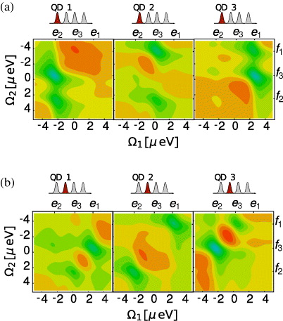
Figure 4. Decomposition of the imaginary part of the DQCS signal with t3 = 20 ps via localization. Part (a) shows spectra with a localized excitation of the first pulse at each QD and part (b) shows a localized second pulse. The detection frequencies are given as detuning around the single and the double gap frequency, respectively.
Download figure:
Standard imageThe single exciton state e1 is mainly connected to the third QD. State e1 has strong transitions to f1 and f3. This way, we already gain new information, which would not be possible without localization of the exciting pulses.
3.4. Localization of the first and second pulses
We can also localize the second pulse for the application of our algorithms; therefore we insert for this interaction the local form of the electron light interaction Hamiltonian, equation (13). For the additional localized field at QD j for the second pulse, we use again perfect localization Eloc2,j(rl) = Eloc2δj,l and obtain

with
and
still under the assumption of a localization of the first pulse at QD i.
Using this localization scheme, we can decompose each of the three plots with a localization of the first pulses of figure 4(a) in three plots with also the second pulse localized. In figure 5, we can see the contribution of the QDs to the single exciton to two-exciton transition μef, connected to their contribution to the ground state to single exciton transition. If we focus on the case with the first pulse mainly exciting QD 1 (first row), we see that the peak at e2 with f3 is mainly visible for a second pulse at QD 3 (and much smaller for a localization at QD 2). On the other hand, with the first pulse mainly exciting QD 3 we see that the peak at e1 and f3 is mainly visible for a localization of the second pulse at QD 1. Therefore, we can conclude f3 that the mainly contributing local two exciton is a state with an excited QD 1 and QD 3. Also the second and the third row show which QD is connected to which single exciton to two-exciton transition of the corresponding spectra of figure 4(a).

Figure 5. Imaginary part of the localized DQCS signal with t3 = 20 ps with realistic localization. While the rows show which QD is excited by the first pulse, the columns give the QD excited by the second pulse. The spectra can be seen as a decomposition of the imaginary part of the full spectrum in figure 3(a) (right). The detection frequencies are given as detuning around the single and double gap frequencies, respectively.
Download figure:
Standard imageIn principle, we can see that, in the case of not too strong coupling and thus low delocalization, figure 5 shows from which local single excitons the two excitons |ij〉 localized at QD i and j are formed.
3.5. Localization of the second pulse
Next, we will show that for reconstructing the two-exciton wave function (see section 3.6.3) it is sufficient to localize the second pulse only. Then, the signal reads

with
and
The first pulse excites all QDs equally in a far field like the third and fourth pulses.
In figure 4(b), spectra calculated with equation (16) are presented. They represent—opposite to figure 4(a)—the decompositions of the imaginary part using a localization of the second pulse of the far-field spectrum. Here, the two-exciton states cannot be assigned to a certain QD in such a simple way as in the exciton case, since the signal is proportional to cekcf*kjμ*gj·Eloc2,j(ωfe) and thus to a product of the single and two-exciton wave functions. As expected already from the spectrum with two localized pulses, the main part of the resonance at e2 with f3 originates from QD 3, whereas the main part of the resonance at e1 with f3 originates from QD 1. Thus f3 is mainly composed of e1 and e2, which are primarily located at QD 3 and QD 1, respectively. In a similar way, we see that f1 has contributions from e1 and e3 mainly localized at QD 2 and QD 3.
3.6. Reconstruction of the wave functions
Localized spectroscopy allows several new applications, since spectroscopic data can be used to obtain more information about coupled nanostructures. In this section, we briefly review a protocol to reconstruct the wave functions of single exciton states, first introduced in [26], and extend this to two-exciton states in coupled nanosystems. Section 3.7 presents a filtering method, which is important for enhancing the algorithms used for the reconstruction and supplements this first introductory section.
If the expansion coefficients cei (single exciton wave functions) and cfij (two-exciton wave functions) of equation (2), respectively, are known, it is possible to reconstruct the many particle wave functions |e〉 and |f〉. Additionally, the wave functions of the excited state |i〉 of the isolated emitter i must be known for a full reconstruction. The amplitude and phase of the coefficients c represent how the delocalized wave function is spread over the different QDs. The main idea behind the reconstruction of the wave functions is that spatiotemporal control of electronic fields enables us to eliminate the sum over the QDs i. 2D DQCS, on the other hand, enables us to select specific single and two-exciton states e and f spectrally to remove the summation over e and f. These two techniques allow us to find the coefficients cei for a single exciton state e for QD i and cfij for a two-exciton state f for QDs i and j. In the following, we present a calculation and measurement instruction for reconstructing the wave function for a certain single exciton state  and a certain two-exciton state
  .
.
3.6.1. Single exciton states
In this section, we summarize briefly the method introduced in [26]. For reconstructing the wave function  , we have to select only the contribution from the spectroscopic signal of a specific single exciton state
  . We achieve this by extracting the DQCS signal around the frequencies
  and
and  , where
  is chosen such that the signal has only a strong contribution connected to
  . For this, the spectral contributions of other delocalized states are well separated in the DQCS signal from this resonance. Then, the only contributions of the sum over e and f are terms with
  and
and  . We look at the localized signal for
  at a fixed time interval T3:

with
and
The only part of this signal that depends on the selective excitation of QD i is  . Since both Liouville diagrams share the same interaction at the first step, all other parts do not depend on i. Thus, for the coefficient cei a proportionality relation5 holds:

Assuming that all dipole moments μ*gi for the single exciton transitions and the localized field  are known, we can extract from equation (18) all coefficients
  except for a proportionality factor A. From the normalization of the wave functions we find that
 , so that the coefficient can be determined (except for an arbitrary phase) and the three wave function coefficients are thus reconstructed. To summarize the method for reconstructing the single exciton wave function, we need as input information the dipole moments μgi for all QDs i. In the measurement, we first select frequencies
  and
and  with a main contribution by the single exciton state
  to be reconstructed. Then DQCS signal
  is recorded for all QDs i. In postprocessing the expansion coefficient of the exciton wave function
  are obtained
  , where A is found by the normalization of the wave function
  :
:  .
.
3.6.2. Determining and enhancing the quality of the reconstructed single exciton states
In table 1, all original single exciton states that belong to the chosen example can be compared with the reconstructed values. We find that e1 is the state with the best reconstruction. Furthermore, the best reconstruction is reached choosing the energy of the two-excitonic state f3 to ground state transition for Ω2. This is because that peak has the lowest influence from other resonances (cf the spectrum in figure 3(a)). For the same reason, we choose for the reconstruction of e2 the resonance with f3 and of e3 the resonance with f1.
Table 1. Comparison of the original (O) with the reconstructed (R) single exciton wave function coefficients for a shifted measurement point using a perfect localization: The phase is written in multiples of 2π. The error is calculated via  . Additionally, the results of a measurement point at the center of the resonance are given (C). A reconstruction after filtering e2 is marked with (F) and a reconstruction after filtering states e1 and e2 (FF).
| State | Type | |ce1| | |ce2| | |ce3| | arg(ce1) | arg(ce2) | arg(ce3) | Error |
|---|---|---|---|---|---|---|---|---|
| e1 | O | 0.115 | 0.104 | 0.988 | 0.500 | 0.500 | 0.000 | |
| R | 0.205 | 0.081 | 0.975 | 0.414 | 0.190 | 0.710 | 0.04 | |
| C | 0.247 | 0.077 | 0.966 | 0.433 | 0.281 | 0.787 | 0.06 | |
| e2 | O | 0.977 | 0.169 | 0.131 | 0.500 | 0.500 | 0.500 | |
| R | 0.949 | 0.110 | 0.294 | 0.836 | 0.820 | 0.952 | 0.09 | |
| F | 0.969 | 0.138 | 0.205 | 0.845 | 0.858 | 0.650 | 0.03 | |
| C | 0.969 | 0.136 | 0.206 | 0.725 | 0.680 | 0.907 | 0.03 | |
| e3 | O | 0.180 | 0.980 | 0.083 | 0.000 | 0.500 | 0.500 | |
| R | 0.360 | 0.858 | 0.366 | 0.342 | 0.792 | 0.903 | 0.28 | |
| F | 0.381 | 0.920 | 0.093 | 0.316 | 0.794 | 0.968 | 0.16 | |
| FF | 0.138 | 0.987 | 0.081 | 0.302 | 0.796 | 0.873 | 0.02 |
We measured the quality in terms of the squared error  of the difference of the original wave function coefficient corgi and the reconstructed one creci. This way of error determination does not consider the phase, but it has the most physical meaning since the square of the coefficient gives information about the occupation probability.6
We can still improve the quality of reconstruction of ce1i by moving the measurement point spectrally in the direction of higher single exciton energies, since then we decrease the influence of other resonances.7 This works well mostly except for reconstructing state e2. Also, one would assume that moving the measurement point in the negative Ω1 direction improves the reconstruction quality. But in this special case, interferences of positive and negative contributions are destructive on the right-hand side of the strong peak (e2, f3) and so the influence of other resonances decreases moving to higher energies. Another idea for increasing the quality of reconstruction is averaging over an area of measurement points or additional weighting the results with a Gaussian centered at the main resonance peak; however, this is beyond the scope of this paper. Additionally, we compared in table 1 the reconstruction for choosing Ω1, Ω2 at the center of the resonances.
Reconstructing the exciton wave functions shows overall good agreement for both the amplitude and the relative phase. The values of the resonance with the highest oscillator strength are exemplary illustrated in figure 6.

Figure 6. Coefficients for reconstructing the wave function for the states with a high oscillator strength: above, the original and the reconstructed state with and without filtering of ce2i are presented, whereas below, the original and the reconstructed two-exciton wave function coefficients are shown. Filtering shows a small improvement here.
Download figure:
Standard image3.6.3. Two-exciton states
Similar to the procedure for single excitons, the two-exciton wave functions can also be reconstructed. As a prerequisite, the single exciton reconstruction has to be completed and cei must be known for all single excitons (except for a global phase factor) connected to the two-exciton state.
Here, we use the signal with a localized second pulsed (equation (16)). We select a single exciton state  and a two-exciton state
  ; then
  is the signal with localized second pulses evaluated for frequencies
  and
and  for which mainly
  and
and  contribute (
 and
and  ). We start with rewriting the signal with localized second pulse (equation (16)) just for one selected single exciton state
  and one selected two-exciton state
  as explained in section 3.6.1 and obtain

with
and
We can use the appearance of the factors  in the signal as the starting point for being able to derive an equation analogous to equation (18) for the extraction of two-exciton wave functions. We can reformulate this by introducing proportionality factors
  , which do not depend on localization:

Here, the factor  combines all parts that do not depend on k or j; the form of equation (19) should again not depend on the dephasing model. But as a substantial difference to the single exciton case, we have several factors
  multiplied with single and two-exciton wave function coefficients under a sum over k and j.
Therefore, the next step for isolating the two-exciton wave function  would be isolating the single exciton wave function
  on the left-hand side of equation (19). But we have to recognize that the other factors
  and
and  depend also on the single and two-exciton states, so we cannot apply the orthogonality relation like in the single exciton case. Dividing by
  before applying the orthogonality relation is no alternative, since these factors are unknown and should consequently not appear on the right-hand side. Instead of calculating
  for every e', we compute the ratio of the factor of two arbitrary exciton states: for this we multiply equation (19) with
  and sum over j and obtain

Exchanging  and
and  and the index k with j on the left-hand side and using that cf*kj = cf*jk yields
so that by dividing the two equations we obtain the ratio

This is the first ingredient in the reconstruction, which can be calculated by the measured or derived quantities for each combination of two arbitrary single exciton states  and
and  . In order to remove factors
  on the left side, we choose again another arbitrary exciton state
  and multiply equation (19) by
  and divide by
  to obtain

Here the complete right side of equation (21) is known; one contribution is the measurable spectrum, the single exciton coefficients and the ratio  , which can be calculated using the measured data and equation (20).
Since  does not depend on
  , we can now calculate the two-exciton wave function by multiplying equation (21) with
  and summing over
  . This leads to an orthogonality relation and we obtain

We can now use that the expansion coefficients have been normalized and use  to obtain the two-exciton wave functions of coupled QDs.
After deriving the procedure, we summarize the steps necessary for the reconstruction. As input information we need the dipole moments matrix elements μgi for all QDs i and the single excitonic wave function coefficients cei for all single exciton states. As measurement the DQCS signal with a localized second pulse at QD j
 has to be recorded. In postprocessing, we first calculate the ratios
  for all combinations of single exciton states. Then
  is calculated via
  . Afterwards
  is normalized, using the two-exciton wave function normalization condition
  . So that we can calculate
  up to a global phase.
The results of reconstructing the two-exciton wave functions are shown in table 2. An illustration can be found in figure 6. Again, original states and reconstructed values agree, but not as well as for the exciton state. We can always determine which local two-exciton states contribute most to the delocalized two-exciton state. But crosstalk between the different resonances makes it difficult (cf the reconstruction for f1) to determine the quantitative contribution of the less contributing local two-exciton states, whereas for the other two two-exciton states the agreement is much more acceptable.
Table 2. Comparison of the original (O) with the reconstructed two-exciton wave function coefficients for a shifted measurement point in (R). The data marked with (F) uses filtered spectra for the reconstruction. Additionally, the results of a measurement point at the center of the resonance for all single exciton states are given (C). For all calculations a perfect localization was assumed. The phase is written in multiples of 2π.
| State | Type | |cf12| | |cf13| | |cf23| | φ(cf12) | φ(cf13) | φ(cf23) | Error |
|---|---|---|---|---|---|---|---|---|
| f1 | O | 0.093 | 0.118 | 0.989 | 0.500 | 0.500 | 0.000 | |
| R | 0.089 | 0.332 | 0.939 | 0.349 | 0.789 | 0.503 | 0.14 | |
| F | 0.244 | 0.367 | 0.898 | 0.852 | 0.819 | 0.525 | 0.22 | |
| C | 0.140 | 0.377 | 0.915 | 0.313 | 0.709 | 0.424 | 0.19 | |
| f2 | O | 0.988 | 0.113 | 0.106 | 0.500 | 0.500 | 0.500 | |
| R | 0.793 | 0.586 | 0.166 | 0.762 | 0.508 | 0.684 | 0.48 | |
| F | 0.845 | 0.507 | 0.171 | 0.628 | 0.400 | 0.347 | 0.36 | |
| C | 0.778 | 0.601 | 0.184 | 0.705 | 0.424 | 0.257 | 0.51 | |
| f3 | O | 0.124 | 0.987 | 0.106 | 0.000 | 0.500 | 0.500 | |
| R | 0.273 | 0.935 | 0.225 | 0.981 | 0.544 | 0.358 | 0.12 | |
| F | 0.201 | 0.946 | 0.256 | 0.879 | 0.580 | 0.364 | 0.10 | |
| C | 0.297 | 0.921 | 0.253 | 0.879 | 0.464 | 0.270 | 0.15 |
The overall reason for this is that the two-exciton wave functions are calculated using the single exciton wave functions: the errors in obtaining the single exciton wave function are cumulated in the two-exciton wave function. Furthermore, for the reconstruction of the two-exciton wave function the spectrum localized at the second pulse enters not only for one combination of Ω1 and Ω2 but for every single exciton; this also increases the possible errors. This leads to an overall reduced quality of the reconstructed two-exciton wave function.
3.7. Filtering different resonances
In [26], it was shown that a 2D spectrum with the first pulses localized allows to remove certain resonances using postprocessing of the spectra. Since most of the errors in the reconstruction is caused by overlapping resonances, this might enhance the reconstruction of the exciton states.
We will recapitulate the procedure, modified for the extraction process of the coefficients. For this, we note that the spectra equations (14), (16) and (15) have the form of a sum over individual contributions he for different exciton states e:
where the functions he can be calculated from the measured 2D spectrum:
In the construction of  , we exploited a scalar product, which was constructed by multiplying equation (22) with
  and summing over i and using the orthogonality of the delocalized states.
Using this formula, we can filter in postprocessing all resonances to which a certain ground state g to single exciton  transition contributes during the first pulse. The filtered spectra can be calculated as
In figure 3(b), for each resonance a filtered spectrum is presented; we can clearly see that the corresponding resonances are removed from spectra. Therefore it is expected that using the filtered version (out filtering of the already reconstructed states) of the spectrum can clearly enhance further reconstruction of exciton states.
Here, we try to investigate if the filtered spectrum is improving the quality of the reconstructed coefficients. The filtering improves the quality of the reconstructed wave function as can be seen from the error rates for the reconstructed wave function using a filtered spectrum in tables 1 and 2.
As discussed in section 3.6.1, we find the best reconstruction for e1 and the second best for e2, since e1 dominates the spectrum. This is the reason why we used, while reconstructing the exciton state e2, a spectrum with filtering the state e1 out. For the exciton state e3 we filter two states, since the states e1 and e2 are now known. We do not get better values for every single QD, but there is still an overall improvement visible. The results show that filtering can reduce the error of the reconstruction of single excitons (see table 1) at least by a factor of 2 and in the case of the weak resonance e3 by an order of magnitude.
Since one can determine all exciton states, filtering all the single exciton states is possible for reconstructing the two-exciton states. Again, the filtering technique supplies results for most coefficients at a higher quality as can be seen in table 2. But the improvement is not as high as in the case of single excitons, since we have no available filtering for the two-exciton part.
4. Applicability of the reconstruction
The presented methods are not limited to the example of coupled self-organized GaAs/InAs dots. In principle, they are applicable to any system of coupled emitters with two dominant levels contributing to the optical response describable by the Hamiltonian from equation (1). Such systems include colloidal QDs, coupled chromophores, J-aggregates, plasmons in coupled metal nanoparticles, as long as a suitable spatial localization technique for optical fields exists. In order to form the detuning of the individual emitter transition frequency should be smaller or the same order of magnitude as the dipole–dipole coupling—but big enough to separate exciton states.
Additionally, prerequisites apply to the couplings; the dipole couplings between the emitters should be greater than the linewidth of the resonances (dephasing time) in order to be able to separate the delocalized states in frequency space.
Generalization to emitters with more than two levels is possible although the accessible properties might be reduced.
5. Conclusion
In conclusion, we can reconstruct delocalized exciton wave functions of coupled QDs by finding the expansion coefficients of the basis representation. Single particle wave functions of one QD serve as the basis for the single exciton states and two-exciton states serve as two-exciton basis. These prefactors are found with the help of localized spectroscopy.
We have presented protocols for reconstructing delocalized wave functions for exciton states as well as for two-exciton states. The quality of reconstruction depends among other factors on the quality of spatiotemporal control and on influences of neighbor resonances in the frequency domain. Filtering methods can, furthermore, reduce unwanted influences of resonances and thus improve the quality of reconstruction.
Acknowledgments
We gratefully acknowledge support from the Deutsche Forschungsgemeinschaft (DFG) through SPP 1391 (MR and FeS) and SFB 910 (AK). MR also acknowledges support from the Alexander von Humboldt Foundation through the Feodor-Lynen program. SM gratefully acknowledges support from NSF grant CHE-1058791, DARPA BAA-10-40 QUBE and the Chemical Sciences, Geosciences and Biosciences Division, Office of Basic Energy Sciences, Office of Science, (US) Department of Energy (DOE).
Footnotes
- 4
For the following calculations we choose as parameters for the model system:
0 = 0 μeV, 1 = −2.2 μeV, 2 = 0.2 μeV, 3 = 2.5 μeV, VF12 = −0.4 μeV, VF13 = −0.6 μeV, VF23 = −0.3 μeV, V12 = −0.4 μeV, V13 = 0.2 μeV and V23 = 0.8 μeV. - 5
Note: although we assumed a Lorentzian broadening in our equations, this proportionality should not depend on this choice.
- 6
Reconstructed after filtering states e 1 and e2
- 7
The measurement points located near the resonance peak (shifted for better reconstruction) is given via ωe1 g = 2.60 μeV (ωe1 g = 3.12 μeV), ωe2 g = −2.35 μeV (ωe2 g = −3.20 μeV) and ωe3 g = 0.25 μeV. For the corresponding two-exciton measurement points we have ωf1 g = 3.60 μeV and ωf3 g = 0.49 μeV.