Avoiding selection bias in gravitational wave astronomy

Future generations of ground-based gravitational wave (GW) detectors, such as the under-construction Advanced LIGO [1], Advanced Virgo [2] and Kagra [3] or the proposed Einstein Telescope [4], are expected to detect a multitude of GW sources in the coming years [5]. The analysis of these first detected signals will help to answer questions about the rate of binary coalescence [6] and the astrophysical distribution of neutron star and black hole masses [7]. As the number of observed sources increases, it will be possible to use populations of GW sources to perform cosmological parameter estimation [8–11] and to test general relativity [12–14]. Previous searches for GWs have used a hierarchical pipeline based on a detection statistic, with a threshold applied to this quantity to reduce the amount of data to be processed by later stages of the pipeline [15, 16]. Because of the very low amplitude of the expected signals relative to the detector noise level, this process eliminates signals which fail to reach the threshold as well as background noise, amounting to a selection of the loudest events from all the true signals. Any analysis which attempts to draw inferences from a population of signals or events which have been chosen in this way is vulnerable to selection bias if the population of detected signals does not match that of the underlying sources. We draw a careful distinction between selection bias and biases induced by an incorrect application of prior information [17, 18], as the terms 'Malmquist bias' [19–21] or 'Lutz–Kelker bias' [22] are sometimes used to describe both types of bias.

Many areas of astrophysics are subject to such effects, either by intentional selection or thresholding to reduce the background while performing data analysis, or by limited sensitivity of the instrument (e.g. a flux limited survey [23]). Examples from the literature include searches for Type Ia supernovae (SNIa) [24], gravitational waves (GWs) [16], extra-solar planets [25] and high energy neutrinos [26, 27]; and galaxy cluster surveys [28, 29]. Often the aim is to use the resulting set of observations to infer global parameters of interest, e.g. quantities that characterize the population distribution. In the case of SNIa for example, one may aim to infer cosmological parameters from luminosity distance and redshift measurements. In cosmology, the traditional approach has been to produce unbiased estimators of individual event parameters [30–34] which are then used as input for inference of global quantities. Thresholding has been used to reduce the number of false alarms from a background population to a tolerable level, for example thresholding on radio pulse width is applied to data within the LOFAR NuMoon project [35]. Adrián-Martínez et al [36] apply a threshold on a fitting parameter to optimize the separation of cosmic neutrinos and background for the ANTARES neutrino experiment. In GW searches [37], thresholds are set on the signal-to-noise-ratio (SNR) of an event to reduce the volume of data to be processed before additional cuts are applied to minimize the false alarm rate due to detector noise (which is another example of selection). Candidates from future GW searches will be used as input for inferences on global parameters, such as the parameters of the binary neutron-star (BNS) mass distribution.

It has been previously shown [38], that to avoid bias in the analysis of astronomical data in a signal-dominated environment (i.e. no false alarms), one should account for both the detections and the false dismissals within the experiment. In this paper we provide a prescription for completely avoiding selection bias by extending that approach beyond the signal dominated regime. To do this we must consider the cases of detection and dismissal for all other relevant models, most importantly the noise model. Our approach accounts for the data which are thrown away by the application of the threshold, making no assumption that they contain only noise, nor do we assume that detected events are produced only by true signals. Without this extension, future global inferences from GW signals would be limited to the high-signal regime of [38], which discards all events that do not meet the threshold, resulting in sub-optimal performance. Our method will therefore be useful in extracting the maximum information from a thresholded search, and is also applicable to many other sensitivity-limited analyses. We demonstrate this with an example, where lowering the threshold increases the precision of parameter estimation for the BNS distribution and rate, which remains unbiased despite the presence of false alarms.

Consider an experiment in which many measurements are made, each producing data which may contain potential detections, and which are then compared with a detection threshold. We refer to any measurements which pass the threshold as 'triggers', since in most practical cases we will include one or more noise-only models alongside the true signal model. Any measurements which do not pass the threshold are discarded. These non-trigger cases also carry information about the source population, and one should not assume the lack of a trigger implies the lack of true signal, or vice versa.

We divide the experiment into statistically independent multiple measurements, and denote the outcome of each as D. In practice this might mean dividing a search into multiple time periods. The threshold is set on the measured quantity x, which we will call the 'detection statistic'. In general x may be a maximum-likelihood statistic or simply a direct measurement of a physical parameter value but in all circumstances will be subject to noise.

If the statistic passes a threshold x > x_th a trigger is produced, and the value of x is recorded; we denote this case D⁺, and D = (D⁺,x). If on the other hand x ⩽ x_th, no trigger is produced and no value for x is recorded and D = D⁻. We define $\{\mathcal {H}\}$ as our set of plausible models and must include at least two models with one describing the presence and the other the absence of a signal. In general the method extends to many alternative signal models. When specifying a set of models in this way we allow that any model may be true, and that the trigger has a non-zero probability under all of the models. For any single model $\mathcal {H}$ the likelihood function defining the distribution of the statistic x is expressed as $p(x|\mathcal {H},\boldsymbol {\theta }_{\mathcal {H}},\boldsymbol {\gamma },I)$ where $\boldsymbol {\theta }_{\mathcal {H}}$ are the parameters unique to this model, and γ are the global parameters which are common to all trials (following standard Bayesian notation we use I throughout to represent additional information regarding the experiment, and the global parameters γ). Upon performing the single trial, we are interested in inferring the parameters γ. In the case of a statistic above threshold, D⁺, we can write the posterior distribution on γ as

$$\begin{eqnarray} p(\boldsymbol{\gamma}|D^{+},x,I)&=&\sum_{\{\mathcal{H}\}}p(\boldsymbol{\gamma},\mathcal{H}|D^{+},x,I)\nonumber\\ &=&\frac{p(\boldsymbol{\gamma}|I)}{P(x|I)}\overbrace{\sum_{\{\mathcal{H}\}}p(x|\boldsymbol{\gamma},\mathcal{H},I)P(\mathcal{H}|\boldsymbol{\gamma},I)}^{\mathrm{trigger\, likelihood}\,p(D^{+},x|\boldsymbol{\gamma},I)}\,, \end{eqnarray} \tag{ 1 }$$

where $P(\mathcal {H}|\boldsymbol {\gamma },I)$ represents the prior probability on the model $\mathcal {H}$ conditional on the global parameters. Here we are summing the trigger likelihoods over the set of possible models $\{\mathcal {H}\}$, and we do not assume that the model priors are independent of the global parameters, which will be important when discussing signal abundance and rates. The range of possible models can include those where more than one signal is present in the data. We have used the fact that the probability of a trigger conditional on the value x is strictly equal to H(x − x_th) (where H(x) is the Heaviside step function) which is equal to unity for x > x_th. If the model has local parameters $\boldsymbol {\theta }_{\mathcal {H}}$, we calculate the factor $p(x|\boldsymbol {\gamma },\mathcal {H},I)$, i.e. the likelihood of the data conditional on the model and the global parameters, by marginalization:

$$\begin{equation} p(x|\boldsymbol{\gamma},\mathcal{H},I)=\int\nolimits_{\Theta_{\mathcal{H}}} \mathrm{d}\boldsymbol{\theta}_{\mathcal{H}} p(x|\boldsymbol{\theta}_{\mathcal{H}},\boldsymbol{\gamma},\mathcal{H},I)p(\boldsymbol{\theta}_{\mathcal{H}}|\boldsymbol{\gamma},\mathcal{H},I), \end{equation} \tag{ 2 }$$

where $\Theta _{\mathcal {H}}$ is the local parameter space associated with the local parameter $\theta _{\mathcal {H}}$ and the model $\mathcal {H}$. Note that we do not modify this likelihood function to reflect our knowledge of the threshold.

In the alternative case D⁻ where we discarded the specific value of x, we do still know that x ⩽ x_th. For a non-trigger we can therefore write the posterior probability on γ (analogous to equation (1)) as

$$\begin{equation} p(\boldsymbol{\gamma}|D^{-},I)=\frac{p(\boldsymbol{\gamma}|I)}{P(D^{-}|I)}\overbrace{\sum_{\{\mathcal{H}\}}P(D^{-}|\boldsymbol{\gamma},\mathcal{H},I)P(\mathcal{H}|\boldsymbol{\gamma},I)}^{\mathrm{non\mbox{-}trigger\,likelihood}\,p(D^{-}|\boldsymbol{\gamma},I)}\,. \end{equation} \tag{ 3 }$$

As the value of x is unknown the posterior on γ must be marginalized over both the local parameters $\boldsymbol {\theta }_{\mathcal {H}}$ and the unknown data x in the range x ⩽ x_th. Therefore only the information D⁻ appears in the likelihood of a non-trigger conditional on the model and the global parameters:

$$\begin{eqnarray} P(D^{-}|\boldsymbol{\gamma},\mathcal{H},I)&=&\int\nolimits_{\Theta_{\mathcal{H}}}\mathrm{d}\boldsymbol{\theta}_{\mathcal{H}}\int\nolimits_{x{\leqslant}x_{\mathrm{th}}}\mathrm{d}x~p(x|\boldsymbol{\theta}_{\mathcal{H}},\boldsymbol{\gamma},\mathcal{H},I)p(\boldsymbol{\theta}_{\mathcal{H}}|\boldsymbol{\gamma},\mathcal{H},I).\nonumber \\ \end{eqnarray} \tag{ 4 }$$

The quantity derived in equation (4) is related to what is known as the selection function or detection efficiency, defined as the probability of a trigger given the true signal parameters for a given signal model. Here it appears in a modified form: the probability of a non-trigger given a set of global parameters and a model. It is only in this term that the detection threshold x_th actually appears. In practice this quantity (just like the detection efficiency) can be difficult to estimate in some cases.

2.1. An ensemble of trials

Using equations (1) and (3) together with Bayes' theorem we are able to isolate the single trial likelihood functions (identified by the over-braces) in both the trigger and non-trigger cases, P(D⁺,x|γ,I) and p(D⁻|γ,I) respectively. We can now also consider analysing an ensemble of N trials denoted as {D}, where we index each D_i using i∈(1,N). The posterior probability for the global parameters after N independent trials are performed is simply

$$\begin{equation} p(\boldsymbol{\gamma}|\{D\},I)=\frac{p(\boldsymbol{\gamma}|I)}{P(\{D\}|I)}\prod\limits_{i=1}^{N}p(D_i|\boldsymbol{\gamma},I). \end{equation} \tag{ 5 }$$

We can further decompose this expression into trigger D⁺ and non-trigger D⁻ factors,

$$\begin{equation} p(\boldsymbol{\gamma}|\{D\},I)=\frac{p(\boldsymbol{\gamma}|I)}{P(\{D\}|I)}\prod_{j=1}^{n}p(D^{+},x_{j}|\boldsymbol{\gamma},I_{j})\prod\limits_{k=1}^{N-n}P(D^{-}|\boldsymbol{\gamma},I_{k}), \end{equation} \tag{ 6 }$$

where j and k index the n triggers and the N − n non-triggers respectively, and I_j, I_k allow for different background information (such as time-varying detector sensitivity) in each measurement.

We now focus on the common case where there are only two possible models: the presence ($\mathcal {H}^{+}$) or absence ($\mathcal {H}^{-}$) of a single signal per trial. We can reach this case in practice by considering a trial to be a period of time where the probability of >1 signal is arbitrarily small. Equation (6) becomes

$$\begin{eqnarray} &&\fl p(\boldsymbol{\gamma}|\{D\},I)=\frac{p(\boldsymbol{\gamma}|I)}{P(\{D\}|I)}\nonumber\\ &&\times\prod\limits_{j=1}^{n}\left[p(D^{+},x_{j}|\boldsymbol{\gamma},\mathcal{H}^{+},I_{j})P(\mathcal{H}^{+}|\boldsymbol{\gamma},I_{j})+p(D^{+},x_{j}|\boldsymbol{\gamma},\mathcal{H}^{-},I_{j})P(\mathcal{H}^{-}|\boldsymbol{\gamma},I_{j})\right]\nonumber\\ &&\times\prod\limits_{k=1}^{N-n}\left[P(D^{-}|\boldsymbol{\gamma},\mathcal{H}^{+},I_{k})P(\mathcal{H}^{+}|\boldsymbol{\gamma},I_{k})+P(D^{-}|\boldsymbol{\gamma},\mathcal{H}^{-},I_{k})P(\mathcal{H}^{-}|\boldsymbol{\gamma},I_{k})\right]. \end{eqnarray} \tag{ 7 }$$

To relate this to more standard statistical terms, consider the key components which make up the expression, each of which are in reference to single trials:

• $p(D^{+},x_{j}|\boldsymbol {\gamma },\mathcal {H}^{+},I_{j})$ is the likelihood of producing a trigger with statistic value x_j when a signal is truly present.
• $p(D^{+},x_{j}|\boldsymbol {\gamma },\mathcal {H}^{-},I_{j})$ is the likelihood of producing a trigger with statistic value x_j from only the background distribution.
• $P(D^{-}|\boldsymbol {\gamma },\mathcal {H}^{+},I_{k})$ is the likelihood that a true signal does not produce a trigger, i.e. the false dismissal likelihood (or 1 − detection efficiency).
• $P(D^{-}|\boldsymbol {\gamma },\mathcal {H}^{-},I_{k})$ is the likelihood that no trigger is produced when no signal is present, i.e. the true dismissal likelihood.

The abundance or true rate of signal events is important in the two model case, when the two models are for a single signal and background. As the two models give a complete description of the data, we can write $P(\mathcal {H}^{+}|\boldsymbol {\gamma },I)=1-P(\mathcal {H}^{-}|\boldsymbol {\gamma },I)$. The actual rate of signals, or a quantity from which it can be derived, must be included as one of the global parameters γ, and if it is not known then it can be estimated from the ensemble of trials. This makes the prior probabilities for the models dependent on the global parameters γ, so the joint posterior distribution for the rate will not in general be separable from the rest of global parameters. Alternatively, if the true rate of signals is known, it can be substituted into these expressions instead. However, using incorrect assumptions about the rate parameter will therefore bias inference on other global parameters.

The key idea of our approach (in terms best suited to the two model problem) is to use the true and false dismissal probabilities to incorporate the information from the absence of triggers. This requires that these quantities be either calculated or measured. Without these, any observations which can produce non-triggers risk being either biased or sub-optimal and may require ad hoc corrections. It is only by acknowledging and accounting for ignorance that we can derive the correct results. Equation (7) contains all the parts necessary to infer global parameters without bias, making full use of the information that is kept, and accounting for that which is deliberately (or necessarily) discarded.

Searches for GWs signals from compact binary coalescences employ a threshold when selecting which triggers to keep, and so astrophysical statements drawn from these observations will be subject to selection effects [37]. To show how our method can be used to avoid bias, we will consider a toy model in which a GW detector searches for BNSs, and we want to infer the global parameters: the event rate per unit co-moving volume R, and the mean μ_m and standard deviation σ_m of the component mass distribution. We assume that the population of component masses is governed by a Gaussian distribution, and that a single trial constitutes an all-sky search over the duration Δt = 60 s. For each trial, the data comprises a measurement of the SNR ρ and estimates of the component masses m = (m₁,m₂) of any event that exceeds the SNR threshold ρ_th. In reality, the SNR (our detection statistic) is generated through matched filtering of the data. This process includes both analytical maximization of the SNR over one or more of the local nuisance parameters e.g. phase at coalescence, and numerical maximization over a bank of templates on the component mass space. For simplicity, we assume the component mass estimates to be noise free exact measurements although in practice there will be some uncertainty in their values. In addition we ignore the complications associated with the template bank search over the component mass space noting that in practice, maximization of a detection statistic over a bank of templates would act to modify the distribution of the detection statistic for both the signal and noise models. Although our model is simple and lacks the detail of real observations, it will serve to show the salient points of the method.

We suppose that events arise through either a signal model $\mathcal {H}^{+}$ or through a noise model $\mathcal {H}^{-}$. According to the signal model we define the expected (optimal) SNR-squared of a source as

$$\begin{equation} \rho_{\mathrm{opt}}^{2} = \frac{5\pi^{-4/3}}{96}\frac{\mathcal{M}^{5/3}}{d_{\mathrm{L}}^{2}}\int_{20}^{1500}\frac{f^{-7/3}}{S_{h}(f)}\mathrm{d}f, \end{equation} \tag{ 8 }$$

where the chirp-mass $\mathcal {M}=M\eta ^{3/5}$ with the total mass M = m₁ + m₂ and the symmetric mass ratio η = m₁m₂/M². The luminosity distance is given by d_L and the detector noise spectral density is denoted by S_h(f) for which we use the anticipated Advanced LIGO noise curve [39]. Under the signal model, we assume that the measured SNR-squared is drawn from a non-central χ² distribution with two degrees of freedom and a non-centrality parameter ρ²_opt. The component masses are generated from the prior distributions governed by the global parameters μ_m,σ_m and are measured without noise. Under the noise model, we assume the measured SNR-squared is drawn from a central χ² distribution with two degrees of freedom and should be interpreted as arising from detector noise. All data recorded above the SNR threshold due to the noise model will have corresponding component mass measurements drawn from a uniform distribution of masses within our prior search range defined as $\mathcal {S}_{m}\in (0.9M_{\odot },1.8M_{\odot })$. Hence, a noise model trigger will be associated with any possible component mass configuration with equal probability, unlike the signal model events that follow the astrophysical prior distribution. In practice the distribution of inferred masses caused by the noise background will follow its own distribution which can be modelled or measured.

We assume a uniform distribution of sources in volume giving a prior distribution on the luminosity distance of p(d_L|γ,I) = 3d²_L/(d^max_L)³. We have used d^max_L = 600 Mpc, chosen to be beyond the distance at which BNS systems will be detectable, and ignored cosmological effects since the reach of Advanced LIGO is z ∼ 0.05 for BNSs. We simulate 1 year of trials with a true astrophysical event rate (per unit volume per unit observation time) of R = 10⁻⁷ Mpc⁻³ yr⁻¹ with component mass distribution parameters μ_m = 1.2M_⊙ and σ_m = 0.1M_⊙.

First consider the probability of obtaining a non-trigger per trial under the assumption of the signal model $\mathcal {H}^{+}$,

$$\begin{eqnarray} P(D^{-}|\boldsymbol{\gamma},\mathcal{H}^{+},I)&=&\int\nolimits_{0}^{\rho_{\mathrm{th}}^2}\mathrm{d}x\int\nolimits_{\mathcal{S}^{2}_{m}}\mathrm{ d}\mathbf{m}'~p(x,\mathbf{m}'|\boldsymbol{\gamma},\mathcal{H}^{+},I)\nonumber\\ &=&\int\nolimits_{0}^{\rho_{\mathrm{th}}^{2}}\mathrm{ d}x\,\frac{1}{2}\exp\left(-\frac{1}{2}\left[x+\rho_{\mathrm{opt}}^{2}(\mathbf{m})\right]\right)I_{0}\left(x\rho_{\mathrm{opt}}(\mathbf{m})\right), \end{eqnarray} \tag{ 9 }$$

where I₀ is a modified Bessel function of the first kind and x,m' represents the unknown true squared SNR and unknown true component masses over which we marginalize. The complementary quantity, the probability density associated with detection for the signal model, for the jth trial is

$$\begin{eqnarray} p(\rho^{2}_{j},\mathbf{m}_{j}|\boldsymbol{\gamma},\mathcal{H}^{+},I)&=&\int\nolimits_{\mathcal{S}^{2}_{m}}\mathrm{ d}\mathbf{m}'~p(\rho^{2}_{j},\mathbf{m}_{j},\mathbf{m}'|\boldsymbol{\gamma},\mathcal{H}^{+},I)\nonumber\\ &=&\frac{1}{2}\exp\left\{-\frac{1}{2}\left(\rho^{2}_{j}+\rho_{\mathrm{opt}}^{2}(\mathbf{m}_{j})\right)\right\}I_{0}\left(x\rho_{\mathrm{opt}}(\mathbf{m}_{j})\right), \end{eqnarray} \tag{ 10 }$$

where we have used $p(\mathbf {m}|\mathbf {m}',\boldsymbol {\gamma },\mathcal {H}^{+},I) = \delta (m_{1}-m'_{1})\delta (m_{2}-m'_{2})$ since the mass measurements are noise free in this example. For non-trigger and trigger cases under the noise model we have

$$\begin{eqnarray} P(D^{-}|\boldsymbol{\gamma},\mathcal{H}^{-},I)&=&\int\nolimits_{0}^{\rho_{\mathrm{th}}^2}\mathrm{d}x \int\nolimits_{\mathcal{S}^{2}_{m}}\mathrm{ d}\mathbf{m}'~p(x,\mathbf{m}'|\boldsymbol{\gamma},\mathcal{H}^{-},I)\nonumber\\ &=&1 - \exp\left(-\rho_{\mathrm{th}}^{2}/2\right), \end{eqnarray} \tag{ 11 }$$

$$\begin{eqnarray} p(\rho^{2}_{j},\mathbf{m}_{j}|\boldsymbol{\gamma},\mathcal{H}^{-},I)&=&\int\nolimits_{\mathcal{S}^{2}_{m}}\mathrm{d}\mathbf{m}'~p(\rho^{2}_{j},\mathbf{m}_{j},\mathbf{m}'|\boldsymbol{\gamma},\mathcal{H}^{-},I)\nonumber\\ &=&\frac{1}{2\Delta m^2}\exp\left(-\rho_{\mathrm{th}}^{2}/2\right), \end{eqnarray} \tag{ 12 }$$

where Δm = 0.9M_⊙ is the prior range of component masses and we have used the noise model component mass prior distribution $p(\mathbf {m}'|\boldsymbol {\gamma },\mathcal {H}^{-},I) = 1/\Delta m^{2}$. This is also equal to the noise model component mass likelihood $p(\mathbf {m}|\mathbf {m}',\boldsymbol {\gamma },\mathcal {H}^{-},I)$. We define the model priors assuming that Δt is sufficiently small that within a volume V , $P(\mathcal {H}^{+}|\boldsymbol {\gamma },I)=RV\Delta {}t \ll 1$, so $P(\mathcal {H}^{-}|\boldsymbol {\gamma },I)=1-RV\Delta {}t$.

In figure 1 we show the joint posterior probability on the global parameters μ_m and σ_m for a set of different SNR threshold values. The model can be made more complicated by including any number of extra parameters, global or local, e.g. cosmological parameters or the nuisance parameters of individual sources. As the threshold is decreased we increase the number of triggers due to signal events but also increase the number of false alarms (triggers due to noise events). For the case where ρ_th = 8 the number of false alarms is zero but for ρ_th = 4.3 the number of false alarms is nearly equal to the number of true alarms (see figure caption for details). The solid contours in figure 1 show the results of applying our method to the data where it can be seen that decreasing the threshold and correctly accounting for the increase in true and false alarms improves parameter estimation accuracy whilst remaining consistent with the correct parameter values.

Zoom In Zoom Out Reset image size

An additional result is included in dashed grey lines showing the biases that can occur when failing to incorporate all relevant information into an analysis. This incorrect result is calculated by evaluating equation (10) for each trigger and therefore ignores the information contained within both the model prior and the non-triggers. Although it performs as expected when the threshold is high enough to allow no false alarms, the subsequent global parameter estimates become strongly biased for both mass parameters as the threshold decreases and the false alarm rate increases. This analysis assumes that the wider distribution of masses caused by the noise model reflects the real signals, leading to an overestimate of the mass standard deviation. The mean mass is also overestimated since the average mass measurement due to the noise model is equal to the centre of the mass prior range which in this case is higher than the true value. The specific behaviour depends on the nature of the signal, background, and the (incorrect) assumptions that are made, but this is illustrative of the approach implicitly taken by those studies which assume that a given set of GW triggers will all be due to the signal model.

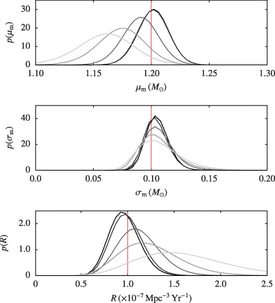
We also show the precision of the global parameter estimates as a function of the threshold value. This is seen in figure 2 where the marginalized posterior distributions on the global parameters including the rate R are plotted for a range of threshold values. We see that the posterior distributions become narrower as the threshold is decreased where more signals and noise events are recorded above threshold. We stress that this improvement in the precision of global parameter estimation is unbiased by the presence of false alarms. This is only true when triggers, non-triggers, signal model, and the noise model are correctly incorporated in the construction of the global parameter posteriors. It is also notable that the reduction in posterior width does not continue linearly with the reduction in threshold or with the corresponding increase in false alarms. In fact, further decreasing the threshold yields diminishing improvements, and the resulting distribution asymptotically approaches the optimal one which would be obtained by removing the threshold altogether. In that case the presence of noise still limits the precision attainable even though all the data is analysed and none discarded. This indicates that there exists a sensible choice of threshold value at which additional computation expense in processing triggers from lower thresholds returns little information. It also implies that operating at thresholds corresponding to high false alarm values will yield the most precise parameter estimates.

Zoom In Zoom Out Reset image size

We have derived a general formalism for analysing data which have been subjected to a threshold, which accounts for both the knowledge of and the ignorance of the actual result of an experiment. This formalism was applied to a simplified real-world example problem from the field of GW data analysis which will be encountered when sufficient detections have been made. The method succeeds for any number of false alarms and reduces to known formulae in limiting cases, such as zero false alarm rate [38]. We find that knowledge of the true rate or abundance of signals represents crucial information when making inferences with an ensemble of trials, and that it can therefore be inferred from them. Prior knowledge of signal and noise models must be incorporated, but measured values of efficiency and false alarm rates can be used when they are difficult to derive analytically.

Our work has implications for research which uses sets of GW signals to probe astrophysical, cosmological, or gravitational parameters, of the kind which have already been suggested in the literature [8–14]. We have shown that the best global parameter estimates will come from using the lowest threshold allowed by computational limitations, which will include using events which were (probably) generated by the background noise.

Our method could be applied in many other noise-limited fields of research, ranging from particle physics to cosmology.

The authors are grateful to J Clark, T Dent, S Fairhurst, I Harrison, M Hendry, D Keitel, T G F Li, W Del Pozzo, G Pratten, R Prix, C Röver, B S Sathyaprakash, P Sutton, M Vallisneri, C Van Den Broeck and G Woan for useful discussions and comments. JV is supported by the research programme of the Foundation for Fundamental Research on Matter (FOM), which is partially supported by the Netherlands Organisation for Scientific Research (NWO). CM is funded by the Science and Technology Facilities Council (STFC) Grant No. ST/J000345/1.