


Abstract
A novel anomalous Nernst effect in graphene engineered by a strain and coupled to an environment with a broken time-reversal breaking is predicted. We consider the Haldane model (1988 Phys. Rev. Lett. 61 2015) including a uniaxial strain and analyze explicitly the time-reversal symmetry behavior. We find in this case that the total Nernst coefficient contributed by the two Dirac cones is no longer zero. For further insight we study the interplay of the stagger-field-induced gap of the substrate and the time-reversal symmetry-breaking-induced gap. The former preserves the opposite signs of the Berry curvatures, whereas in the latter the Berry curvatures possess the same sign. For a weak time reversal breaking (TRB), the total Nernst signal experiences a sign change as the Fermi level increases. When TRB is large, the total Nernst coefficient exhibits a two-peak structure varying with the Fermi level. Another feature is that the anomalous Nernst signal has an anti-symmetric profile with respect to the neutral Dirac point instead of the symmetric behavior known for the case of an external magnetic field. We further find a robust six-leaf modulation of the total Nernst coefficient as the direction of the strain is varied.
Export citation and abstract BibTeX RIS

Content from this work may be used under the terms of the Creative Commons Attribution 3.0 licence. Any further distribution of this work must maintain attribution to the author(s) and the title of the work, journal citation and DOI.
1. Introduction
The usual Nernst effect is a thermomagnetic phenomenon of a triggered electric current transverse to a temperature gradient and an external magnetic field applied perpendicular to both the temperature gradient and the charge current [1]. This effect is currently discussed as a sensitive probe in the context of high-Tc superconductivity [2] and also for graphene-based systems, e.g. monolayer graphene [3, 4] and graphite [5]. Owing to the Dirac fermion character in graphene, the Nernst coefficient deviates markedly from the Mott relation for the n = 0 Landau level (LL) around the Dirac point [3, 4]. Theoretically this deviation is yet to be fully understood [3]. On the other hand, the Nernst effect goes along with the quantum Hall effect which is inherent for a topologically protected edge current. The number of edge states is just the Chern–Simon number (or the winding number) which is given by an integral over the Berry curvature on the momentum torus for the two-dimensional (2D) Brillouin zone (BZ) with periodic boundary. The difference between the Hall conductance and the Nernst coefficient is that the latter is determined not only by the Berry curvature but also by the entropy generation around the Fermi surface. Therefore, the Nernst effect is sensitive to the change of the Fermi energy, the temperature and other quantities. The common feature of these two effects is that in an external electric field the charge carrier attains an extra anomalous velocity with ℏvk = eE × ΩνK(K')z, where E is the electric field, ΩνK(K')z is the Berry curvature, ν = 1 (2) stands for the conduction (valence) band and K (K') indicates the Dirac cone located at K (K') (see figure 1(b)). Hence, a finite Berry curvature may lead to an anomalous Nernst effect in the absence of an external magnetic field which is the case discussed here.
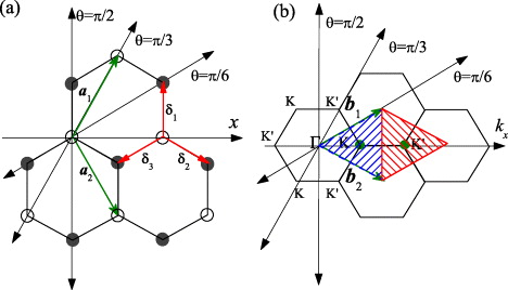
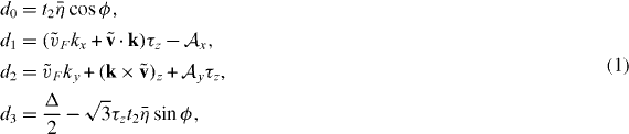
Figure 1. (a) Graphene crystal structure is shown. a1 and a2 are primitive vectors. (b) The first BZ is shown. The shaded regions correspond to the regions for K and K' cone. b1 and b2 are primitive vectors in the momentum space.
Download figure:
Standard image High-resolution imageFor gapless graphene [6], the Berry curvature shows a singularity at the Dirac points so that the Berry phases ±π are associated with the two Dirac cones. A substrate-induced gap (hereafter referred as the substrate gap) was observed experimentally when a SiC substrate is used [7] and in an ab initio calculation with a BN substrate [8]. For the graphene layer, such a substrate gap yields a finite Berry curvature for each cone. However, these Berry curvatures have opposite signs [9, 10]. In a recent study, we showed that in a time-reversal symmetry (TRS)-breaking environment, strain can lead to an anomalous Hall effect [11].
Since both the quantum Hall effect and the Nernst effect are intrinsically linked to the topology of the momentum space, it is interesting to investigate how to engineer the topology of the Dirac cones of graphene. In this respect, the strain is currently intensely studied [12]. It is expected, however, that the strain-induced static electric potential does not break the TRS. To study whether the TRS is still maintained in an essentially transient non-equilibrium transport (e.g. Nernst effect when strain builds up) is out of the scope of this paper [13]4. Here, we consider a specific model that provides an explicit TRS breaking. We study a graphene layer on a 'Haldane' substrate under a uniaxial strain. The substrate effect is described within a Haldane-type model [14, 15], i.e. a zero flux through one unit cell but with a vector potential structure. The Haldane model takes the next-nearest-neighbor hopping into account and leads to massive Dirac fermions. The nearest-neighbor hopping leads to coupling to the planar motion of Dirac fermions. In this work, we will show that a novel anomalous Nernst effect emerges and can be engineered by the strain. In contrast to the case without strain [10], the total Nernst coefficient (TNC) does not vanish and undergoes a sign change when increasing an applied gate voltage (for a small flux). We found a robust six-leaf geometry of the TNC as a function of the angle of the strain with respect to the zigzag direction.
2. The model
The Pauli matrices σ1 = σx and σ2 = σy represent the E representation of C3v group at the Dirac points of graphene and are related to the A and B sublattice character. σx and σy indicate that there is a coupling between A and B sublattices which can be in the lowest order provided by the nearest-neighbor hopping, while σ3 = σz essentially describes the breaking of this sublattice degeneracy and gives rise to mass generation of the Dirac fermion. This mass can be generated by a stagger field due to the static electric interaction with the substrate. For example, if the substrate has a honeycomb structure (or from a top view is felt by the Dirac fermions in the graphene layer), but the two atoms in the unit cell are not equivalent, then a staggered field acts on the two carbon atoms in the unit cell of the graphene. This coupling generates a mass of the Dirac fermion and enters into the coupling to σ3. Another contribution entering the coupling to σ3 is the TRS breaking term in the Haldane model. The Haldane TRS breaking term is a consequence of an extra phase due to the next-nearest-neighbor hopping. The low-energy effective Hamiltonian is written as H = σ·d(k). From the theory of invariants [16], we obtain the d vector in the K and K' cones without including explicitly the external electric field
where  is the energy gap induced by the stagger field of the substrate (substrate gap), τz denotes the valley degree,
  ,
,  ,
,  ,
,  is a dimensionless function varying with strain, δt2i is the variation induced by strain to the next-nearest-neighbor hopping labeled by i = 1,2,3 and ϕ is the flux of the effective magnetic field generated by the substrate (see the appendices). We should point out that the d0 and d3 terms are derived by the next-nearest-neighbor hopping (hopping in the same sublattice) and the d1 and d2 terms are obtained from the nearest-neighbor hopping (hopping between different sublattices). Furthermore, we introduced the strain tensor as defined in the continuous elastic theory as
  , where u is a polar vector indicating the displacements of atoms. In principle, all the bij parameters can be determined experimentally or from ab initio calculations [16] in a similar manner as done for semiconductors. Another way is to link these parameters to those derived from tight-binding formalism. This is obviously a transparent and effective approach to connect with microscopic method. However, this way is not explored thoroughly for graphene. For example, the case to study the deformed next-nearest-neighbor hopping is still missing, to our knowledge. For the effect of the deformed nearest-neighbor hopping, research is being undertaken extensively. If only the deformed nearest-neighbor hopping integrals are taken into account [17, 18], one finds an effective gauge field that is independent of the momentum. Recently, it was pointed out that the strain influence should be envisaged by including the effects of the deformed lattice in the real space, the deformed momentum vectors and also the deformed hopping integrals [19]. After expanding the Hamiltonian around the Dirac points, extra terms can be obtained which may be momentum-dependent. This changes definitely the topology of the Dirac cones. A corresponding effect is, however, still unexplored for the next-nearest-neighbor case. To that end and for the purpose of our study, we worked out an effective Hamiltonian in tight-binding formalism for this case and obtained a concrete model with a TRS breaking under strain in appendix B.
Thus, every term in equation (1) can be determined by tight-binding parameters and finally determined by solely the strain tensor. In this way, the model is well founded and its parameters are linked in a transparent way to microscopic quantities.  and
and  are to be viewed as effective vector potentials in a minimal coupling scheme for the strain-induced transport [17, 18]. It is instructive to recall that the vector potential is expressible in terms of the hopping parameters in a tight-binding formalism
  and
and  , where
  , i = 1,2,3, are the variation of the nearest-neighbor hopping integrals induced by the strain with respect to the change of the nearest-neighbor vectors δi shown in appendix D (a similar expression was given in [20]). Thus, the essential feature is that vector d mediates a map from a 2D momentum space to a three-dimensional vector space. We will study the consequences of this mapping beyond the minimal coupling.
Without strain, the cross section of the Fermi level and the Dirac cone is a circle (for Ef is not exactly at the Dirac point). Upon including the strain, this circular topology of the cones is changed into an ellipsoidal ring. Gaps are opened at the original Dirac points at K and K'. However the positions of the minimal energy gap are no longer located at these original Dirac points, they are floating elsewhere when changing the strain since the strain serves in effect as a magnetic field in the momentum space and the Dirac points can be regarded as monopoles in the same space. To capture this behavior, we use the linearized momentum with respect to the original Dirac points. In the absence of strain, the Hamiltonian reduces to the linear Hamiltonian around these points. To study the Nernst effect carefully, we have to use all the components in the first BZ. Thus, we use a rhombic BZ marked by the shaded regions in figure 1(b). In this way, the number of states in the BZ is conserved after linearization of the spectrum around the Dirac points, which is as an alternative to the usual Debye prescription [21].
To be specific, we consider throughout the work a uniaxial strain only. The x direction is selected as the zigzag direction; the momentum space x direction (kx) is shown in figure 1. The angle of the applied tension with respect to x direction is θ. We first calculate the energy contour for the conduction band in the presence of the strain, as shown in figures 2(a) and (b). First of all, we observe that the circular Dirac cone is deformed to an elliptical cone for both K and K' cones. The original Dirac points are shifted away by the strain since the strain effect serves partly as a gauge field in the momentum space. For zero gap graphene, the Dirac points are monopoles in the BZ. Although there is a gap considered here, they should be affected by the induced gauge field. Although the TRS breaking in the model studied here is based on the Haldane model, it is instructive to think about some other situations with a possible TRS breaking. The TRS breaking environment could be created by applying a weak magnetic field in the graphene sheet so that the orbital motion and the Zeeman effect can be ignored. Graphene easily wrinkles into the third dimension with nanometer-scale ripples that have been observed in microscopic studies [22]. The existence of the rippling has been demonstrated to be not only extrinsic, e.g. by surface roughness of the substrate, but also intrinsic in graphene [23]. Therefore, an in-plane magnetic field induces additionally a random magnetic field both in the xy direction and z direction [24–26]. TRS is expected not to be present at all. Alternatively, the graphene layer may be put on a magnetic substrate to break the TRS. In this case, a non-vanishing effect enters into the third component of the d vector. This is reflected by the asymmetric K and K' in figures 2(a) and (b) since different gaps are opened in addition to the uniform gap  . It is useful to recall that another mechanism to break the TRS might be having spontaneous microscopic currents due to the order parameter of a density wave as that in the context of underdoped cuprate superconductor where a square lattice is considered [27, 28].
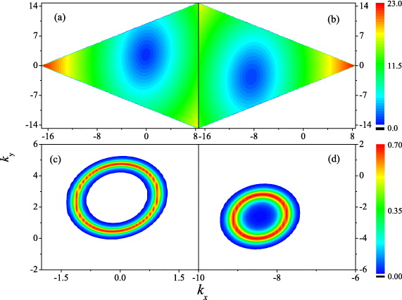
Figure 2. Energy contour for the conduction bands in BZ for K cone in (a) and K' cone in (b); the entropy density for K and K' cones in (c) and (d), respectively. The units of the wave vector and the energy are k0 = 1 nm−1 and  . The parameters in all graphs are
  and
and  = 0.1. The temperature is 300 K and the Fermi energy is Ef = 1.2 eV in (c) and (d).
Download figure:
Standard image High-resolution image3. Nernst coefficient in the strained graphene
What we intend to study is an anomalous Nernst effect that emerges for a non-vanishing Berry curvature. This Berry curvature manifests itself in an additional anomalous velocity term in the presence of an external electric field ℏvk = eE × Ω. Thus, the velocity multiplied by the entropy density gives rise to the Nernst coefficient [10, 27]

where α0 = ekB/h, e is the electron charge, kB is the Boltzmann constant, ℏ is the Planck constant and n = K or K', ν = + 1 (−1) for the conduction (valence) band, Sν(k) = −fνk ln fνk − (1 − fνk) ln (1 − fνk) is the entropy density of the ν band and fνk = f[Eν(k)] is the Fermi distribution function. Please note that equation (2) yields the Nernst coefficient for one cone. The integral over k should be taken in the respective triangle BZ shown in figure 1(b).
In figures 2(c) and (d), the entropy density is calculated for the K and K' cones for Ef = 1.2 eV. Different from the energy contour, the entropy density displays a maximum around the Fermi energy. The ellipsoidal topology is clearly seen from the maximum of the entropy density, as well. Another observation is that TRS breaking is observed in the symmetry breaking of the two Dirac cones. This can be inferred from the values of the entropy density and the different positions of the shifted Dirac points in the momentum space.
It has been shown in [11] that the Berry curvatures for the two cones have the same signs rather than opposite signs in the absence of the gap Δ, but in a TRS breaking environment. Therefore, the anomalous transverse velocities will be the same for the two cones leading to a net Hall current driven by an external electric field. It is natural to expect that an anomalous Nernst coefficient will be associated with this anomalous transverse velocity. In figures 3(a) and (b), TNC which is the sum of the contributions from the two Dirac cones is calculated while varying the Fermi level for the different magnetic fluxes and the strain magnitudes in figures 3(a) and (b), respectively.
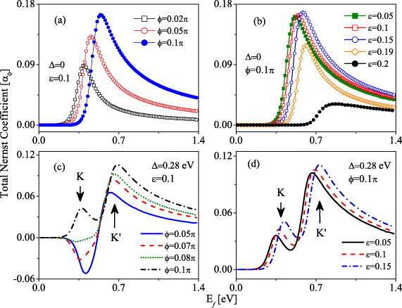
Figure 3. The Nernst coefficient is calculated as a function of the Fermi energy for different fluxes and strains in (a), (c) and in (b), (d), respectively. The temperature is T = 300 and the direction angle of the strain is θ = π/4. Δ = 0 for (a) and (b), while Δ = 0.28 eV for (c) and (d).
Download figure:
Standard image High-resolution imageThe peak in the TNC when the Fermi level lies in the conduction band can be understood as follows. The Nernst coefficient is affected by two factors. (a) The Berry curvature which exhibits a maximum value at the Dirac points or the bottom of the conduction band. (b) The maximum of the entropy density is, however, around the Fermi level leading to a finite-width Fermi ring in the momentum space. Thus, when the Fermi level increases, the area of the entropy density in the momentum space increases; while the Berry curvature decreases. The overall effect manifests itself as a peak of the Nernst coefficient. The peak shift induced by the flux and the strain is a consequence of increasing the asymmetry of the energy and the gaps in the two cones (see figure 2(a)). It is interesting to note that the magnitude of the peak of the TNC is first enhanced slightly by increasing the strain from a small distortion and then is decreased by a strong strain (see figure 3(b)).
When the gap Δ is present, the behavior of the Nernst coefficient is determined by the relative magnitudes of this gap and the gap induced by the TRS breaking which is affected by the strain. Hereafter we call the gap Δ the stagger field gap (SFG) and the latter the time-reversal-breaking (TRB) gap. When SFG is dominant, the Berry curvatures for the two Dirac cones are of the opposite signs. Since the total gaps at the two Dirac points are asymmetric, one cone yields at first a dominant contribution to the Nernst signal when the Fermi level is touching the band edge of this cone. When further increasing the Fermi level, the other cone will affect the Nernst signal by reducing it due to the opposite signs of the Berry curvatures of the two cones. This explains the marked difference and even the sign change shown in figure 3(c). However, when the TRB gap is enlarged with larger flux, the Berry curvature of one cone (K) is gradually converted by its sign. This makes the negative TNC turn to a positive TNC at K point. When the TRB gap is dominant, the signs of the Berry curvatures for the two cones are the same, leading to a two-peak structure of the TNC varying with the Fermi level. In figure 3(d), the peaks of the TNC are shifted to a larger Fermi energy with increasing the strain in accordance with the enlarged total gap.
We shall compare the behavior of the Nernst signal in the whole gate voltage range, scanning the case when the Fermi level both in the conduction band and the valence band. Since both SFG and TRB gaps do not change the particle–hole nature of the conduction and valence bands, the Berry curvatures take opposite signs for these two bands. Therefore, the sign of the Nernst coefficient is anti-symmetric with respect to the neutral Dirac point. This is in complete contrast to the case when applying a magnetic field. In the presence of an external magnetic field, Landau quantized orbits are formed. The Nernst signal is [3]

where β = (kBT)−1 and En indicates the energy of nth LL. The Nernst signal shows peaks near the LLs, while it tends to zero in between the LLs [29, 30]. This gives rise to a symmetric profile of the Nernst signal when crossing the Dirac point due to the symmetric distribution of the LLs with respect to the Dirac point. This distinctive symmetry difference indicates the different nature of the case studied here to the physics under an external magnetic field.
In figure 4, the variation of the TNC with the strain angle is shown for zero Δ, finite Δ and different strain cases. The graph exhibits a six-leaf geometry as we vary θ. The maxima are all located at θ = 0°, 60°, 120°, 180°, 240° and 300° (for the selected Ef = 0.7 eV). In between the maxima the Nernst coefficient turns six minima at θ = 30°, 90°, 150°, 210°, 270° and 330° (a few directions, i.e. θ = π/6, π/3 and π/2, are shown explicitly in figure 1). The positions of the maxima and minima of the Nernst coefficients are robust against varying the parameters of the system, such as ε, the SFG Δ and the Fermi levels. It is interesting to note that the directions where the Nernst coefficients attain maxima pass through the two Dirac points, while the TNC is minimal when the strain is along the primitive vectors in the momentum space and σd1, σd2 and σd3 in the C3v group for the Dirac cones [31]. Estimating the order of the obtained TNC we note that α0 ≈ 3.33 nA K−1 corresponds to 100 μV K−1 of a quantum resistivity  . Thus, 10−2α0 corresponds to 1000 nV K−1, which might be measurable.
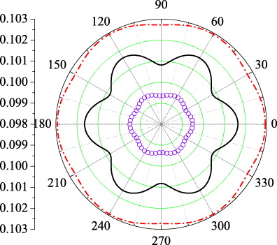
Figure 4. The TNC varies with θ, which is the angle between the direction of tensile strain and the zigzag direction. The parameters for the solid line are ε = 0.1, Δ = 0; the data are multiplied by 0.9. The parameters for the dash-dot line are ε = 0.05, Δ = 0. The parameters for the line with open circles are ε = 0.05, Δ = 0.28 eV. The other parameters are σ = 0.165, T = 300 K and Ef = 0.7 eV.
Download figure:
Standard image High-resolution image4. Summary
We demonstrated that a novel anomalous Nernst effect driven by an external electric field rather a magnetic field can be induced in strained graphene coupled to a TRB environment. The Haldane model under strain is studied as a specific illustration. We investigated the action of the Berry curvatures of the two Dirac cones and how it is changed by strain. The interplay of the stagger-field-induced gap of the substrate and the TRS-breaking-induced gap is studied. The former preserves the opposite signs of the Berry curvatures, whereas the latter renders the same signs of the Berry curvatures. For weak TRS breaking, the total Nernst signal experiences a sign change when the Fermi level is elevated. When the TRB gap is large, TNC shows a two-peak structure with varying Fermi level. This sign change does not occur if only the SFG is missing. Hence, this effect may serve as a thermal-electric probe for the existence of such a gap. We found a robust six-leaf configuration of the TNC as the angle of the strain varies with respect to the zigzag direction.
Acknowledgments
We thank C L Jia, K-H Ding and V K Dugaev for useful discussions. JB was supported by DFG. ZGZ was supported by DFG-SFB 762, and is now supported by Hundred Talents Program of The Chinese Academy of Sciences.
Appendix A.: Haldane model without strain
The Hamiltonian including the second nearest-neighbor hopping reads

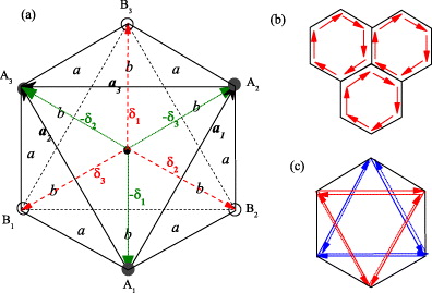
A is the vector potential in the Haldane model, the integrals in the exponents are to be performed along the paths connected by the atoms located at Ra(b)i and Ra(b)j for A (B) sublattice. A method to construct a Wigner–Seitz (WS) unit cell is shown in figure A.1(a) in which a hollow position is selected as the starting ends of primitive vectors. Therefore, each atom among the six atoms located at the corners of the honeycomb belongs to three WS unit cells and there are two atoms effectively in one WS unit cell. The vectors δi are the three vectors connecting the nearest neighbors. a1 = δ1 − δ3 and a2 = δ1 − δ2 are two primitive vectors; in addition a3 = δ3 − δ2. Since the hollow position is labeled by Ri for the ith WS unit cell, the locations of the six atoms are
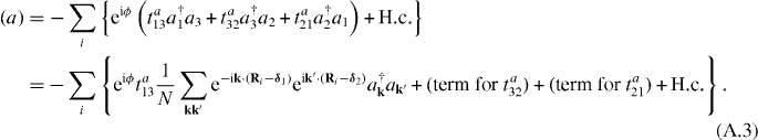
Figure A.1. Schematic figure of a Wigner–Seitz unit cell, the nearest hopping flow and the next-nearest-neighbor hopping are shown in (a)–(c), respectively.
Download figure:
Standard image High-resolution image
If we use a vector to indicate the hopping between the carbon atoms (for example ta†b), the reversed vector means a Hermitian conjugate hopping (for example tb†a). For the nearest-neighbor hopping, we only need to write the terms constituting a clockwise loop in one WS unit cell, and the Hermitian conjugate terms will be recovered by doing the same thing in another WS unit cell. From figure A.1(b), we clearly see this and there are two inverse vectors for each nearest 'bond'. For the next-nearest hopping, we need to include both the clockwise and anti-clockwise loops along the two triangles since the next-nearest 'bonds' are not the common edges of the WS unit cells (see figure A.1(c)).
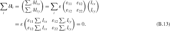
For each sublattice, we can group three terms out of the six terms, and the three terms left are then the Hermitian conjugate of the selected three ones. We select A3 → A2 → A1 → A3 and B1 → B3 → B2 → B1. In the presence of the vector potential, we have  , where S is the area of the honeycomb,
  is the triangle formed by three points located at A1, A2 and A3. The zero flux through the honeycomb has been used for the last equation. Since the field B(r) is supposed to have full symmetry of the crystal, we have
  , where
 ![$\phi =\frac {2\pi }{\phi _{0}}\left [2\Phi _{a}+\Phi _{b}\right ]$](https://content.cld.iop.org/journals/1367-2630/15/7/073028/revision1/nj451820ieqn19.gif) , Φa(b) is the flux through the region labeled by a and b in figure A.1(a).
, Φa(b) is the flux through the region labeled by a and b in figure A.1(a).
The items for A sublattice in the nearest-neighbor hopping are now
We use a relation 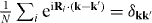 in the above equation, leading to

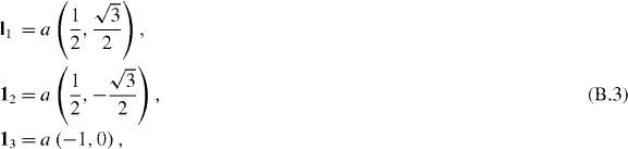
If we define l1 = a1, l2 = −a2 and l3 = a3, we have

For graphene layer without strain, we set all the second nearest hopping to be the same t2. We have then

A similar calculation can be performed for the B sublattice giving rise to
Thus, the Hamiltonian for the next-nearest-neighbor hopping is
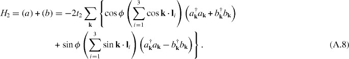
Appendix B.: Haldane model under strain
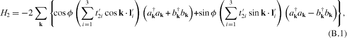
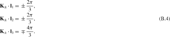
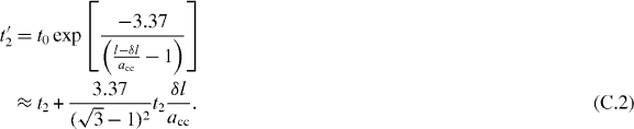
In these appendices, we use K± to indicate K and K'. In the presence of strain, the next-nearest-neighbor hopping is changed, and the vectors li in real space are also deformed. We write explicitly t'2i = t2 + δt2i, where i = 1, 2 and 3 indicate the three next-nearest-neighbor 'bonds'. And we have l'i = li + δli. Under the strain, the Haldane model for the next-nearest-neighbor hopping is
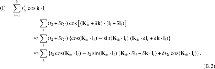
To proceed further we list
where  , acc is the bond length for carbon–carbon atoms. By using
 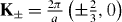 , we have
Therefore, we obtain


Therefore, we find

Similar calculations yield

Since  , we obtain
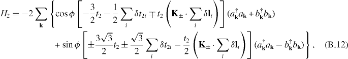
Therefore, we arrive at the Hamiltonian
We consider explicitly uniaxial strain as a study case, and the displacement of the l vectors is given by (see the strain tensor in [17])
With this we infer the Hamiltonian including the next-nearest-neighbor hopping

where  is a dimensionless function varying with strain. The single-particle Hamiltonian reads

Appendix C.: Relation between the variation of the hopping and the variation of the bond length
We use the relation derived in [17]

where t0 is the nearest-neighbor hopping parameter. The deformed next-nearest-neighbor hopping is given by the variation of the length l
Thus, we have

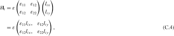
where δt2i is the difference between the deformed t'2 and t2 associated with the vector li. So we have
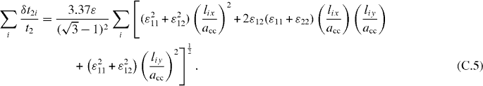
In the case of a uniaxial strain, the strain tensor is given by
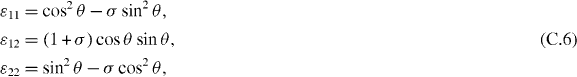
where σ = 0.165 is the Poisson ratio [32] and θ is the angle between the tension direction and the zigzag direction.
Appendix D.: Nearest-neighbor hopping under strain
The Hamiltonian of the nearest-neighbor hopping under strain can be derived as
where κ is the momentum vector with respect to the Γ point,  and
and  is the variation of the hopping integral induced by the strain. In deriving this equation, we have assumed that the BZ is maintained, but the structure in real space and the hopping integrals are deformed. In principle, BZ and the vectors in momentum space are also deformed. In some sense, the distortion of the vectors in momentum space can be compensated by the deformed vectors in real space. Thus, we assume here that the structure in the BZ is not changed for simplicity
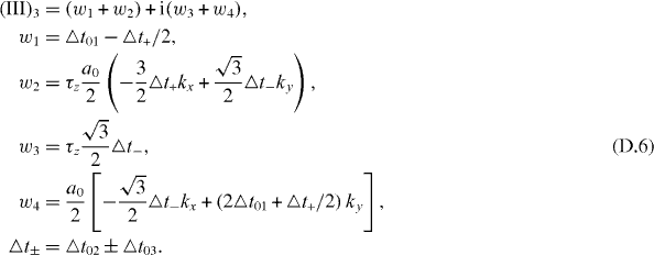
where k is the momentum vector with respect to K±. (III)1 can be derived as usual

where  , a0 is the distance of the carbon–carbon atoms, and t0 is the nearest-neighbor hopping without strain. We have
After some algebra, we have
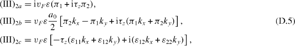
where τz = 1 (−1) for K+ (K−), π1 = K±,xε12 + K±,yε22 and π2 = K±,xε11 + K±,yε12. A straight calculation leads to
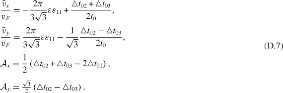
We ignore (III)4 since the lowest order is the second order in a small change and independent of the momentum. If we link the formalism derived in the tight-binding method to that derived from the theory of invariants, we ignore the terms that are independent of kx(y), i.e. (III)2a, and the term including the deformed momentum kx(y), i.e. (III)2c. Then we re-derived the d1 and d2 vectors in (1), and link the parameters in this equation by
 can be calculated as done in appendix C, and we list the equation here

where δix(y) are the x (y) component of the vector δi.
Footnotes
- 4
In non-equilibrium thermal statistics the detailed balance theorem is violated, which means that TRS is broken in this process. For more discussions on TRS breaking in the non-equilibrium case, please see [13].