


Abstract
This paper describes the theoretical foundation of and explicit algorithms for a novel approach to morphology and anisotropy analysis of complex spatial structure using tensor-valued Minkowski functionals, the so-called Minkowski tensors. Minkowski tensors are generalizations of the well-known scalar Minkowski functionals and are explicitly sensitive to anisotropic aspects of morphology, relevant for example for elastic moduli or permeability of microstructured materials. Here we derive explicit linear-time algorithms to compute these tensorial measures for three-dimensional shapes. These apply to representations of any object that can be represented by a triangulation of its bounding surface; their application is illustrated for the polyhedral Voronoi cellular complexes of jammed sphere configurations and for triangulations of a biopolymer fibre network obtained by confocal microscopy. The paper further bridges the substantial notational and conceptual gap between the different but equivalent approaches to scalar or tensorial Minkowski functionals in mathematics and in physics, hence making the mathematical measure theoretic formalism more readily accessible for future application in the physical sciences.

Content from this work may be used under the terms of the Creative Commons Attribution 3.0 licence. Any further distribution of this work must maintain attribution to the author(s) and the title of the work, journal citation and DOI.
The morphology of complex spatial microstructures is often classified qualitatively into types such as cellular, porous, network-like, fibrous, percolating, periodic, lamellar, hexagonal, disordered, fractal, etc. Various quantitative measures of morphology have been defined, often applicable to one specific type only, for example moments of the distributions of angles of tangent vectors with a fixed specified direction as anisotropy characterization of a network structure. Apart from the concept of correlation functions, few measures are defined sensibly and robustly for all types. In this paper, we describe the class of Minkowski functionals, or Minkowski tensors (MT) for short that apply generically to almost any type of structure that contains two or more phases separated by a well-defined interface, for example, porous media, foams, trabecular bone, granular material. The MT are defined as integrals of powers of normal and position vectors and surface curvatures, or curvature measures. Because of their tensorial nature they are explicitly sensitive to anisotropic and orientational aspects of spatial structure. Figure 1 shows examples of systems where subtle anisotropy of the spatial structure influences the physical properties and to which the analysis of this paper is applicable.

Figure 1. Examples of systems with anisotropic spatial structure. (a) A microphase-separated copolymer film aligns under the influence of an external electric field (image courtesy of Böker and Olszowka, see also [8, 9]). (b) Closed-cell metal foam (image courtesy of Saadatfar [10]). (c) Structure of trabecular bone (image courtesy of Alan Boyde (a.boyde@qmul.ac.uk.)). (d) Packing of ellipsoids as a model system for anisotropic granular matter.
Download figure:
Standard image High-resolution imageThe scope of this paper is the thorough theoretical description of the MT approach to spatial structure analysis and the derivation of a robust algorithm to compute MT of bi-phasic materials. It will facilitate the use of Minkowski tensors as robust structure metrics for shape description and for structure–property correlations in physics and materials science. It simultaneously provides the theoretic and algorithmic basis of our previous applications of this method [1–7], and broadens the scope of the MT concept. A secondary purpose is to bridge the gap between the notation and concepts commonly used in the physics literature for scalar Minkowski functionals (MF), based on surface and volume integrals, and the integral geometry literature, where both scalar and tensorial MF are derived based on measure theory. (Unless specified, the abbreviation MF is henceforth used for the scalar Minkowski functionals.)
MT are direct generalizations of scalar-valued MF. These latter are well established as succinct descriptors of morphology and spatial structure for various physical processes [11]. These integral geometric measures have been applied to disordered porous materials [12] and are relevant to flow phenomena therein [13, 14], to nano-scale microstructures in copolymers [15], to the dewetting dynamics of thin films [16] and to Turing patterns [17]. They have also been shown to be the most pertinent morphological quantities on which the thermodynamic properties of simple fluids near curved solid interfaces depend [18, 19]. The mathematical theory of MF and their generalizations have been comprehensively developed in the context of integral geometry [20–23], with several aspects shared also with the discipline of mathematical morphology [24–26].
MF as scalar quantities are not sensitive to features of the morphology which relate to orientation or directional anisotropy, since motion invariance is one of their defining properties. Therefore, scalar MF do not provide quantification of anisotropy that is relevant to study the direction dependence of physical processes, such as elastic properties or permeability of anisotropic porous or microstructured materials or systems with external fields. This motivates their generalization to tensorial quantities. MT have already been shown to be the relevant morphological descriptors for a density functional theory of fluids of non-spherical particles [27] and of DNA conformations [28], and of a simple model for transport with molecular motors [29]. They have also been used, in two dimensional systems, as morphology descriptors of arrangements of neuronal cells [30], galaxies [31] and Turing patterns [6].
The mathematical discipline of integral geometry has proven statements regarding continuity and completeness similar to the Hadwiger theorem in the scalar case [32–35]. However, an algorithm for the computation of the MT applicable to experimental three-dimensional (3D) data—a prerequisite for their use as shape indices for experimental data—has thus far been lacking. (Note that the work in [1–7] has employed the algorithms described in this paper without thorough description.)
A primary application of rank-2 MT is the quantitative analysis of the degree of intrinsic anisotropy of materials with complex spatial structure. Scalar measures of anisotropy are easily derived as eigenvalue ratios of the MT. Evidently, alternative methods for the characterization of anisotropy and alignment exist. Fourier transforms are a common way to characterize anisotropy, and have been applied, e.g., for trabecular bone [36], for electrodeposited patterns [37], for fibre systems [38] and for structured polyethylene mats [39]. Related methods based on correlation functions are also known [40, 41]. Fourier methods that analyse the amplitude of the Fourier transform of a grey-scale image in polar coordinates can also quantify alignment, e.g. of copolymer films in electric fields [8]. Anisotropy indices derived from the normal vector distribution of a given shape, similar to the MT, have been used to describe the shape anisotropy of simulated 3D foam cells [42, 43] and liquid interfaces [3, 44]. An anisotropy measure applicable to porous media is derived from the directional variations of average chord lengths. For a binary composite, i.e. consisting of a solid and a void phase, a chord is a segment of an infinite straight line that is fully contained in one of the two phases. Analyses of chord lengths and the derived mean intercept length ellipsoid are used for the investigation of the microstructure of bone [45–50], see also [51] for a comparison of anisotropy measures based on mean-intercept length, star-volume and star-length distributions. Deformations of cellular or granular material have recently been quantified using the so-called texture tensor C, defined as the sum over a subset of link vectors l in the structure [52, 53]. The texture tensor can be used to characterize anisotropy, e.g. for Antarctic ice crystals [54] and liquid foam cells [55]. Further anisotropy measures are based on the Steiner compact [56], wavelet analysis [57], the orientation of volumes [58] or star volumes [59]. Two-dimensional equivalents of the anisotropy measures discussed in this paper have previously been used for the analysis of the shape of neuronal cells [30] and galaxies [31], and are discussed in detail in [6].

The paper is organized as follows. Section 1 provides an overview of the theory of MF and MT, based on their definition by surface integrals which is widely used in the physical sciences. To bridge the gap in notation between the physics and the mathematics literature this section also includes a discussion of the alternative definition based on measure theory. Section 2 derives algorithms to compute MT for bodies represented by triangulations of their bounding surface; their implementation is provided as online supplementary data (available from stacks.iop.org/NJP/15/083028/mmedia) to this paper. Section 3 describes anisotropy measures derived from the MT and illustrates their application to two experimental data sets. The appendix provides analytic expressions for the MT for some simple geometric shapes.
1. Definition and fundamental properties
Scalar MF and MT can be used as shape measures to quantify the shape or form of an object. They can be defined in two largely equivalent ways. In the physical sciences, a definition based on curvature-weighted integrals of position or surface normal vectors over the object's bounding surface has been popular for the scalar MF, and forms the basis of the numerical algorithms derived in this paper. An alternative, more fundamental definition is provided by the measure theoretic approach of integral geometry (see section 1.2).
The object, also referred to as body, whose shape can be characterized by MT or MF is denoted by K. Assuming that K is a compact set with non-empty interior embedded in Euclidean space and is bounded by a sufficiently smooth surface ∂K, we define MF of K as


in space dimension d = 3 and with ν = 1,2,3. The scalar functions Gν are G1 = 1, the mean curvature G2 = (k1 + k2)/2 and the Gaussian curvature G3 = k1k2 of the bounding surface ∂K; the scalars k1, k2 are the principal curvatures on ∂K as defined in differential geometry, dV is the infinitesimal volume and dA is the scalar infinitesimal area element. This definition naturally applies to both convex and non-convex bodies of arbitrary topology with a sufficiently smooth bounding surface. The prefactor is chosen such that for a sphere BR with radius R the scalar MF are Wν(BR) = κ3 R3−ν where κ3 = 4π/3 is the volume of the 3D unit sphere4.
The MF W2 and W3 (in 3D space) are not properly defined by equation (1) for bodies with sharp edges or corners, due to singularities of the mean and Gaussian curvatures G2 and G3. However, for convex bodies, consideration of a parallel or dilated body in the limit of vanishing thickness provides a robust definition, by use of the Steiner formula. The Steiner formula states that, for a given convex body K, the MF of the parallel or dilated body () are a polynomial in  ⩾ 0 with coefficients proportional to the MF of K; for > 0, is the parallel or dilated body of K (see figure 2). Specifically for the volume one finds , and more generally


Sharp edges and vertices of K correspond to cylindrical or spherical segments on the bounding surface of the parallel or dilated body. The bounding surface is sufficiently smooth for > 0 and converges to Wν(K) in the limit → 0. It is further necessary to define MF and MT for certain non-convex bodies, with or without positive reach, see e.g. [23, Note 1 to section 5.3 and references therein]; this is achieved below by exploiting an additivity relationship. A further discussion for non-smooth bodies can be found in section 2.


Figure 2. (a) A body K with bounding surface ∂K; (b) a convex polytope P and its parallel body (or dilation) ; (c) a subset of a topologically more complex body based on Craig Marlow's painting 'White Spirits' [60]. The latter demonstrates a common experimental situation, namely that the given body K represents a finite subset of a larger body K+, here the body K is clipped to the window of observation T, K = K+∩T. It is assumed that K is a representative subset of the larger body, which allows for the estimation of intrinsic shape features of K+. If only K, but not K+, is available for analysis, particular care must be taken w.r.t. those bounding surface patches of K that result purely from taking the subset, i.e. those that are on the boundaries of the window of observation.

Download figure:
Standard image High-resolution imageMT are symmetric tensors (that is, invariant under index permutation), which are generated by symmetric tensor products of position vectors x and normal vectors n of ∂K. The dyadic (or tensor) product of two vectors a and b is (a⊗b)ij: = aibj. Let now a and b be symmetric tensors of rank r and s, respectively. The symmetric tensor product is defined as

where Sr+s is the permutation group of r + s elements. For two tensors a and b, we use the shorter notation a2: = a⊙a = a⊗a and ab: = a⊙b. For example, if a and b are both vectors, the symmetric tensor product is the tensor ab of rank 2.
The MT of rank 2 are defined as


with ν = 1,2,3 and (r,s) = (2,0), (1,1) or (0,2). For ease of notation, we set Wr,s0: = 0 for s > 0 and Wr,sν: = 0 if ν < 0 or ν > 3. For a 3D body, this definition yields ten MT, not counting the ones that vanish by definition for all bodies.
MT of rank one (called Minkowski vectors) are defined by and by for ν = 1,2,3. The prefactors are chosen such that, for a sphere centred at C, the so-called curvature centroids W1,0ν/Wν are equal to C. Note specifically that W1,01/W0 is the centre of mass (assuming a solidly filled body of constant density). Formally, vectors W0,1ν proportional to for ν = 1,2,3 are also defined, however they vanish for any body with a closed bounding surface [34].


MT are isometry covariant, that is their behaviour under translations and rotations is given by


where is the translation of K by the vector t, UK is a rotated copy of K and denotes the corresponding rotation tensor for a rank-(r + s) tensor:


In this expression, Uij is the conventional orthogonal 3 × 3 transformation matrix associated with the rotation U.
For r = 0, equation (6) gives . A tensor that fulfils this relation for all K is called translation invariant. Genuinely translation covariant tensors fulfil equation (6) but not the translation invariance condition. For the sake of brevity, we will use the term translation covariant to denote specifically the genuinely translation covariant tensors. All W0,sν are translation invariant by their definition; in dimension d = 3, also the tensors W1,11,W1,12 and W1,13 are translation invariant due to the envelope theorems of Müller [34]. Translation invariance is important whenever a natural choice for the origin is not available.

All MF and MT are homogeneous, i.e. they fulfil the homogeneity relation Wr,sν(λK) = λ3+r−νWr,sν(K). Table 1 specifies the translation and homogeneity behaviour of the MF and MT.
Table 1. Basic tensor valuations in 3D. The MF (scalars, rank 0) are motion invariant and the Minkowski vectors (rank 1) are genuinely translation covariant. For rank two, the space of MT decomposes into two complementary subspaces according to translation behaviour (indicated by the last column): genuinely translation covariant and translation invariant tensors. The latter include tensors obtained by multiplying the scalar MF Wν with the unit tensor Q: = e21 + e22 + e23 of rank 2, where e1,e2,e3 are vectors of an orthonormal basis of .

| Homogeneity (unit) | Rank 0 | Rank 1 | Rank 2 | Translation behaviour |
|---|---|---|---|---|
| λ5 [m5] | – | – | W2,00 | Genuinely translation covariant |
| λ4 [m4] | – | W1,00 | W2,01 | Genuinely translation covariant |
| λ3 [m3] | – | W1,01 | W2,02 | Genuinely translation covariant |
| W0 | – | W0 Q | Translation invariant | |
| λ2 [m2] | – | W1,02 | W2,03 | Genuinely translation covariant |
| – | – | W0,21 | Translation invariant | |
| W1 | – | W1 Q | Translation invariant | |
| λ1 [m1] | – | W1,03 | – | Genuinely translation covariant |
| – | – | W0,22 | Translation invariant | |
| W2 | – | W2 Q | Translation invariant | |
| λ0 [1] | W3 | – | W3 Q | Translation invariant |
Thus far, MT have been defined for (a) convex or non-convex bodies with a smooth bounding surface and (b) convex bodies that may have sharp corners and edges. The case of non-convex bodies with concave sharp corners or edges cannot be treated by the parallel body construction ('dilation') without further assumptions (technically, such bodies do not represent sets of positive reach [23, 61]). An extension of the definition of MF and MT to finite unions of convex bodies is achieved by exploiting a property called additivity

if K, K' are all convex. In general, the union (K∪K') of two arbitrary convex bodies K and K' is not convex while the intersection (K∩K') is convex. Since Wr,sν are continuous functionals on convex bodies, equation (9) can be used (see Groemer's extension theorem [23]) to define the MF and MT for bodies that are unions of a finite number of convex bodies (such sets are called polyconvex).
MT of rank (r + s) with r + s > 1 are not completely linearly independent, i.e. they do not contain independent shape information [33, 62]. For rank-2 MT and d = 3 the linear dependences

are valid for any polyconvex body K in and ν = 0,1,2,3; Q is the unit tensor of rank 2. In particular, it follows that QW3 = 3W0,23. Specifically, for ν = 0 one obtains a special case of the Gauss theorem


and hence W0 = tr W11,1. These relations are special cases of [33, equation (1.1)] or [62, equation (1.5)].
Alesker's theorem [32] makes a strong statement about the completeness of the MT for the purpose of shape description. For the special case of tensors of rank 2, it states that any isometry covariant, additive, continuous functional φ on general convex bodies in , taking values in the space of symmetric tensors of rank 2 over , is a linear combination of the basic tensor valuations (an additive functional is called valuation) QpWr,sν, that is


with real coefficients that do not depend on the convex body K [33, p 150]. The coefficients φr,s,pν vanish unless r + s + 2p = 2. Starting from equation (12) and using the linear dependences among the basic tensor valuations, φ can be expressed in terms of linearly independent basic tensor valuations which form a basis of the corresponding vector space. The vector space of continuous, isometry covariant tensor valuations of rank 2 in has dimension 10. A particular basis of this vector space consists of the six tensor valuations W2,00, W2,01, W2,02, W2,03, W0,21 and W0,22, which contain pertinent independent shape information, and of the four tensor valuations QWν, ν = 0,...,3. A summary is provided in table 1.


Since φ is continuous and additive on convex bodies, it can be extended as an additive functional to finite unions of convex bodies. For this additive extension, equation (12) remains valid since the right-hand side is a linear combination of additive functionals. It should be emphasized, however, that although all of these functionals are continuous on the space of convex bodies, they are not continuous on the space of finite unions of convex bodies, see the example in [6, figure 3].
1.1. Minkowski tensors of convex polytopes
It is instructive to illustrate the MT for convex polytopes P and to point out similarities to the tensor of inertia. We use here the letter P, rather than K, to denote a body whose bounding surface is a triangulation consisting of planar polygonal facets. For a polytope, the tensors W2,0ν characterize the distribution of mass if the cell is a solid cell (W2,00), a hollow cell (W2,01), a wire frame (W2,02) and a cell consisting of points at the vertices only (W2,03); in the last two cases, however, this distribution of mass is weighted with certain exterior angles (see figure 3).
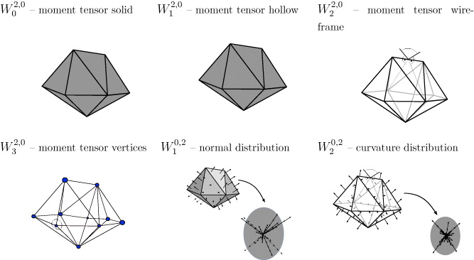
Figure 3. Interpretations of the MT for a polytope P. (Top left) Assuming homogeneous density, W2,00 is the mass distribution tensor. (Top middle to bottom left) contributions to surface-integrated moment tensors W2,0ν with ν = 1,...,3 are concentrated on (3 − ν)-dimensional faces. (Bottom middle and right) moments of the normal distribution on ∂P. Contributions to normal moment tensors W0,2ν with ν = 1,...,2 are also concentrated on (3 − ν)-dimensional surfaces (reproduced from [4], copyright © 2011 Wiley-VCH Verlag GmbH & Co. KGaA, Weinheim).
Download figure:
Standard image High-resolution imageThe tensor of inertia IP, defined by , is a measure of the mass distribution of a (homogeneous) body K, relevant for the relationship between a rotation and the resulting moment. As IP is not translation-covariant, it is not a linear combination of the MT. However the simple relationship holds for arbitrary K; as above Q is the unit tensor of rank 2 of , also called metric tensor. This illustrates that W2,00(K) is a measure of the distribution of mass if K is a homogeneously filled solid, somewhat analogous to the tensor of inertia. Similarly, W2,01(K) characterizes the mass distribution if K is hollow and bounded by an infinitesimally thin surface sheet. This interpretation of W2,00 and W2,01 is valid for bodies K bounded by arbitrary surfaces (not just polytopes).


For a polytope P, the tensor W2,02(P) reduces to a line integral over the edges of the polytope (as the mean curvature vanishes on the flat facets, see also section 2) and is hence related to a mass distribution if P is given by a wire frame with wires along the edges. However, imposed by the requirement of additivity, the weight of the wire cannot be uniform but must be proportional to the mean curvature along the edge (i.e. the dihedral angle). Similarly, the tensor W2,03(P) reduces to a sum of point contributions, as the Gaussian curvature G3 of P vanishes except at the vertices of the given polytope P. Again due to the additivity requirement, these vertices need to be weighted with the Gaussian curvature G3.
1.2. Definition based on fundamental measure theory
This section describes the alternative (and in some sense more fundamental) definition of MF and MT based on integral geometry and fundamental measure theory. The purpose of this section is to bridge the gap between the mathematics and physics literature on MF and MT. However, its content is not required for the numerical approaches to MF and MT described in section 2.
In integral geometry, the definition of MF and MT is based on so-called support measures (sometimes called generalized curvature measures) that can be thought of as local versions of the scalar MF [20, 22, 23, 63].
If support measures are available, then the MT for convex (or more general) bodies are obtained by integrating tensor functions with respect to these measures. Here we describe the approach for convex sets. The idea underlying the introduction of support measures for convex sets is to generalize the notion of a parallel set (or 'dilation', see figure 4 for d = 2) of a convex body K in d-dimensional Euclidean space to a suitable local construction.


Figure 4. Construction of a local parallel set. (a) Definition of the normal field over an arbitrary convex body K at its boundary ∂K. (b1)–(b2) Local parallel set (illustrated for a polytope P) where only points are considered for which the normal direction is in a prescribed subset S of the unit sphere. (Here .)


Download figure:
Standard image High-resolution imageA definition of the local parallel set that also applies to convex bodies K without smooth boundary is given in the following. We define pK(x) as the unique point in K which is nearest to a given point . This defines a continuous map , x↦pK(x). Then dK(x): = ∥x − pK(x)∥ is the distance from x to K and nK(x): = (x − pK(x))/dK(x), for , is an exterior unit normal of K at the boundary point pK(x)∈∂K (see figure 4). This construction achieves a definition of nearest points (reminiscent of the Euclidean distance map [64]) and surface normals that is also well defined for points x whose nearest point on K is a sharp corner (where the tangent plane is not well defined and hence the conventional differential geometric definition of the surface normal does not apply).


Now we shall derive a local Steiner formula and support measures, following [23] to obtain local support measures. The definition of MF and MT then follows directly as a special case [33, 62]. The intuitive idea underlying the definition of a local parallel set is described in two steps. Firstly, we specify a region and some > 0. Then we consider all points which have distance dK(x) at most from K and for which pK(x)∈L. Secondly, if K has points (such as at sharp corners or edges) where the exterior surface unit normal vector is not unique, then it is natural to restrict the points in this local outer parallel set further by also requiring nK(x) to lie in a prescribed set of the unit sphere in . As an example, consider the polytope P in figure 4(b1); for the definition of the local parallel set (shaded dark) it is necessary to specify which angular fraction of the wedges should be part of the local parallel set. This motivates the definition of the local parallel set by specification of the spatial region L and by the subset of normal directions, conveniently combined to . This two-step procedure can be merged and slightly extended to the following general definition.


For given > 0 and , the local parallel set of K defined by


contains all points with 0 < dK(x) ⩽ such that the pair (pK(x),nK(x))∈η. The first condition restricts x to the global outer parallel set (see figure 4(b1)). The second condition restricts to those points of the global outer parallel set, where (pK(x),nK(x))∈η.


The volume of this local parallel set of a convex body K is , where Vd is the d-dimensional Lebesgue-measure. A fundamental result in integral geometry, known as the local Steiner formula [23, 63], states that the map for all > 0 is a polynomial of degree d, that is


where is the volume of an n-dimensional unit ball and Λν(K,η), ν = 0,...,d − 1, are certain real coefficients that depend on K and η, but not on .

For equation (14) to be true for all > 0, it is crucial that K is convex [65]. Equation (14) is easily confirmed (and evaluated) for a convex polytope P. In this case, the set can be decomposed in an elementary way into wedges over the faces F of P as indicated by figure 4(b1). Let denote the ν-dimensional faces of the polytope P5


the set of unit normal vectors assigned to and relint F the relative interior of F (i.e. the interior of F w.r.t. the lowest-dimensional embedding affine hull); see figure 5.


Figure 5. (a) Illustration of the set of normal vectors on the surface of a polytope P. (b) Normal vector assigned to a facet . (c) Line segment of normal vectors assigned to an edge . (d) Spherical triangle/patch of normal vectors assigned to a vertex .


Download figure:
Standard image High-resolution imageThe contributions to coming from each of these wedges


can be calculated by a simple integration known as Fubini's theorem or Cavalieri's principle [66, 67]. This shows that for η = L × S equation (14) holds with

where ων = ν κν is the surface measure of the (ν − 1)-dimensional unit sphere and is the Hausdorff measure of dimension ν [68].

Since an arbitrary convex body K can be approximated by polytopes, equation (14) can be derived by a continuity argument. In fact, Λν(K,η) can be expressed as a linear combination of , for μ > 0 pairwise different and μ = 1,...,d. One obtains an invertible d × d-matrix equation (with the matrix entries d−νμκd−ν) with ν running from 0,...,d − 1. Therefore, the properties of the local parallel volume (in particular, additivity and weak continuity) are also available for Λν(K,η) [63, p 202]. In particular, K↦Λν(K,η) is an additive functional for fixed η. That is, for convex bodies K and K'


Furthermore, η↦Λν(K,η) is a non-negative measure for fixed K. The latter means that if , , is a sequence of mutually disjoint (measurable) sets, then


This property is called σ-additivity of Λν(K,·). Weak continuity of Λν means that for every sequence of convex bodies Kμ , with Kμ → K and every continuous function the equation


holds. Note that this does not imply Λν(Kμ,η) → Λν(K,η) as μ → ∞ for all measurable sets

In particular, Λν(K,·) can be used to integrate functions over . It is plausible that Λν(K,·) is concentrated on the normal bundle . In other words, N(K) consists of all such that n is an exterior unit normal vector of K at x. The measures Λν(K,·), ν = 0,...,d − 1, are called support measures and are determined as coefficient measures of the Steiner formula, equation (14). They are local versions of the classical MF Wν, since .


If K is sufficiently smooth, then

where Gν(x) is the (ν − 1)th (normalized) elementary symmetric function of the principal curvatures of ∂K at x. That is in three dimensions, these are 1, the mean curvature and Gaussian curvature, respectively. 1{·} is the characteristic function, which evaluates to one if its argument is true and 0 otherwise. For general dimensions and ν ⩽ d − 1, equation (21) holds for all sufficiently smooth convex bodies K.
Having introduced the support measures as local versions of the scalar MF, it is easy to define the MT for a convex body K by

hence we obtain Φr,sν(K) by integrating the tensorial function xrns with respect to the measure Λν(K,·) over . If K is a polytope, for d = 3 this yields equation (A.3), up to a different normalization. If K is smooth, we obtain equation (5), up to a different normalization and indexing scheme, i.e.


The notation Φμ,r,s or Φr,sμ for the MT in equation (22) is preferred in some of the mathematical literature and differs from the notation Wr,sν in equations (4) and (5) only by a different indexing scheme and a different normalization. In , i.e. for d = 3, the functionals Φr,sμ and Wr,sν are related by


for ν = 1,...,d, and

The additivity and continuity properties of the support measures immediately yield the corresponding properties of the MT. This approach also shows that if it is possible to define support measures for a class of sets, then the corresponding tensor valuations can be defined by equation (22).
Since the theory of support measures is well developed [23, 63], the measure theoretic approach outlined above has some advantages over the differential geometric approach.
As a simple illustration, let us explain why W1,1d−ν is translation invariant for ν = 0,...,d − 1. Observe that by translation covariance of the support measures

It is a basic property of the measures Λν(K,·) that they are centred at the origin in the sense that [34], which yields the assertion.

A natural and useful extension that is suggested by general measure theory is to introduce local tensor valuations by restricting the integration on the right-hand side of equation (22) to measurable subsets of .

2. Algorithms for bodies bounded by triangulated surfaces
We describe an exact algorithm for all independent scalar, vectorial and rank-2 MT of bodies bounded by piece-wise linear (i.e. triangulated) surfaces. Henceforth such bodies, convex or non-convex, are called polytopes P and their bounding surface is the triangulation . Triangulations are commonly used as discrete approximations of smooth surfaces. The continuity of the MF and MT guarantees the convergence of the formula for the triangulations to the MF and MT of the smooth body.

The formulae are derived for convex bodies with triangulated bounding surfaces by considering parallel bodies P of convex polytopes P (i.e. P has a continuous normal field and finite curvatures for > 0 and a well defined limit as → 0). By application of the additivity relation these formulae are then shown to be valid also for bodies that are not convex. The key results of this paper—explicit formulae for the computation of MT of convex and non-convex polytopes—are summarized in table 2.
Table 2. MF and MT in 3D of body K with smooth boundary ∂K and a body P bounded by a triangulated surface ∂P.
| Scalar measures | ||
| W0 | ||
| W1 | ||
| W2 | ||
| W3 | ||
| Vectorial measures | ||
| (W1,00)i | , see section 2.4 | |
| (W1,01)i | ||
| (W1,02)i | ||
| (W1,03)i | ||
| Tensorial measures (rank two) | ||
| (W2,00)ij | , see section 2.5 | |
| (W2,01)ij | ||
| (W2,02)ij | ||
| (W2,03)ij | ||
| (W0,21)ij | ||
| (W0,22)ij |


Second column. MF and MT for bodies with smooth boundary ∂K. The mean and Gaussian curvatures on ∂K are G2 and G3, respectively. Third column. MF and MT for a triangulation. The set of facets of the triangulation is , the set of oriented edges is (in DCEL structure, see text) and the set of vertices . The subset of triangles that contain the vertex v is denoted by . The nomenclature for triangulated surfaces is defined in figure 6. The vertices of an edge e or a triangle T are denoted v1,v2 and v3, respectively. |T| is the area of , CT its centre point (v1 + v2 + v3)/3 and the tensors IT and JT are given in equations (33) and (35) and table 3. Ce = (v1 + v2)/2 is the centre point of edge e and |e| its length. The letters i,j,k denote tensor or vector indices, with i,j∈{x,y,z} and k according to table 3. The symbol 〈·,·〉 denotes the scalar product. αe is the dihedral angle across edge e, see section 2.2. nT is the normal of triangle T, pointing out of the body, see figure 6. The jump angles ϕvT are defined in section 2.3 and figure 8, and the quantities and below equation (37).


Consider a polytope P in with piece-wise linear bounding surface . Without loss of generality, the linear facets may be assumed to be triangles6 . The set of all triangular patches of ∂P is , the set of oriented edges is and the set of vertices is . We assume a doubly connected edge list (DCEL [69], also called half edge data structure7), that is, every edge which is shared between two triangles T and T' is a double edge consisting of two oriented edges e (being part of T) and e' (part of T'), constituting an unambiguous assignment of each edge to a triangle. Each oriented edge is assigned to its previous edge eprevious and its next edge enext. The remaining ambiguity in the edge orientation is lifted by requiring the triangle normals nT = (eprevious × e)/|eprevious × e| to point out of the body P. Thus, we can uniquely assign to each oriented edge e a triangle T with vertices v1, v2 v3 (see figure 6) and its normal vector nT .


Figure 6. (a) Definition of geometric properties of a triangulated surface ∂P with DCEL. Each edge e is oriented and uniquely assigned to a triangle T. The counter-oriented edge to e is denoted e' and assigned to the adjacent triangle T'. An oriented edge e is unambiguously assigned to the previous edge eprevious and the next edge enext. The normal vector nT is defined to point out of the body K, i.e. nT = (eprevious × e)/|eprevious × e|. The angle between two edges of triangle T at vertex v is denoted ϕvT . (b) Cross-sectional view along an oriented edge e. The normal vectors nT and nT' of the triangle T (that contains e) and T' span the angle αe∈(− π,π]. A concave edge has a negative angle αe. The figure also shows the definition of the local coordinate system used for the computation of W0,22. The basis vectors and are defined as , and . (c) Subdivision of a body P along a concave edge e to yield locally convex bodies.


Download figure:
Standard image High-resolution imageThe parallel body construction is illustrated by figure 2(b). For an arbitrary body P the parallel body P with thickness > 0 is defined as . For a convex polytope P (whose bounding surface has a discontinuous normal field) the bounding surface ∂P has a continuous normal field. The curvatures are patch-wise constant: G2 = G3 = 0 on the planar patches, G2 = (2)−1 and G3 = 0 on the cylindrical patches corresponding to polygon edges, and G2 = 1/ and G3 = 1/2 on the spherical patches corresponding to polytope vertices. For convex polytopes, the MT are defined as the surface integrals of equation (5) evaluated on ∂P in the limit → 0. The result thus obtained is equivalent to equation (22), see also equation (A.3).

2.1. Volume W0
The calculation of the volume of a polytope P can be transformed into a surface integral by the Gauss theorem, see equation (11) and [70]. With div x = div(x,y,z)t = 3 one obtains

where dA = n dA denotes the oriented infinitesimal area element and 〈·,·〉 the scalar product.
2.2. Surface area W1 and integral mean curvature W2
The surface integral is a sum over triangles and is easily evaluated yielding the formulae in table 2. This result is independent whether P is convex or not. The surface area W1(P) of ∂P is simply the sum of triangle areas.
Expressing W2(P) as the limit of vanishing parallel distance of W2(P) of the parallel body P, W2(P) = lim→0W2(P), the contributions of facets vanish because the mean curvature of a flat face is zero. The contribution of the spherical patches S corresponding to vertices vanishes because the integral over a spherical patch S can be parametrized in spherical coordinates by which vanish as → 0. The remaining contribution of the edges is located at the cylindrical patches of ∂P and is given in polar coordinates by


where |e| is the length of edge e and αe the dihedral angle, i.e. the angle between the surface normals of the two facets adjacent to e. For a convex body, all edges have a dihedral angle 0 ⩽ αe ⩽ π; see also figure 6. Note that is the set of oriented edges, i.e. the edge shared by two triangles is represented by two distinct oriented edges, which explains the factor 1/2 in front of the integral.

Equation (28) remains valid even if P is not convex, as is shown by exploiting additivity: a non-convex polytope P can be decomposed into a set of convex polytopes by cutting along the symmetric bisector planes of all concave edges (i.e. −π < αe < 0), see figure 7. For a concave edge e, the symmetric bisector plane is the plane that is spanned by e and the average of the facet normals of the two facets adjacent to e. By adding the contributions of all resulting convex bodies using the additivity relationship equation (9), as outlined in figure 6(c), one obtains the validity of equation (28) for non-convex triangulated bodies. The sign of the dihedral angle αe∈(− π,π] determines whether the edge is convex (αe > 0) or concave (αe < 0).

Figure 7. Subdivision of a non-convex body into convex sub-bodies, P = P1∪P2∪ P3∪P4∪P5. Note that for the computation of MT the segments P2 and P4 need to be taken into account, although their volume measure is 0: W0(P2) = W0(P4) = 0.
Download figure:
Standard image High-resolution image2.3. Integral Gaussian curvature W3 (Euler index χ)
As the point-wise Gaussian curvature G3 on cylinders and flat facets vanishes, only vertices of the triangulation (and their corresponding spherical patches on the parallel body) contribute to W3. For both a convex and a non-convex polytope P the point-wise Gaussian curvature G3 and the integrated Gaussian curvature W3 can be calculated by the well-known simple sum over angle deficits at surface vertices in equation (30), derived below, and also given in [71, 72]. The non-convex case is treated by exploiting additivity.
The Gaussian curvature contribution of the vertices is derived by the Gauss–Bonnet formula


where is the subset of triangles adjacent to vertex v and S denotes the spherical patch on the parallel surface ∂P. For all > 0 each spherical cap S⊂∂P can be uniquely assigned to one vertex v; ∂S its oriented boundary curve and kg the geodesic curvature along ∂S. At the corners of ∂S, the discontinuity of the tangent vectors is characterized by jump angles ϕvT (see figure 8) which for all > 0 coincide with the interior angles of the triangle T at v [73], see figure 8. The geodesic curvature kg vanishes almost everywhere along ∂S, because ∂S are great circle arcs on the spherical patch and the adjacent cylindrical patch and are thus geodesics; hence the integral vanishes.


Figure 8. Sketch of a vertex v with a spherical patch S of the parallel surface ∂P. The interior angle in the triangle T adjacent to v is denoted ϕvT . S is a spherical polygon. The jump angles coincide with the interior angles of the triangles.
Download figure:
Standard image High-resolution imageAs a consequence, is constant for all > 0. Equation (29) therefore yields a definition and an explicit formula for W3(P) as a sum of the local contribution w3(P,v) at a vertex v


At a concave vertex v, a polytope P can always be decomposed into three separate bodies (one of vanishing volume) that have convex vertices in lieu of v. It is easy to validate equation (30) at concave vertices by using the additivity relation in equation (9), see figure 9.

Figure 9. The Gaussian curvature G3 at a saddle vertex is obtained by a virtual decomposition of P at v into three polytopes with vertices vμ, μ = 1,2,3 using the additivity property of MT.
Download figure:
Standard image High-resolution image2.4. Centre of mass W1,00/W0 and curvature centroids W1,0ν/Wν
The Minkowski vector W1,00 corresponds to the centre of mass of P multiplied with its volume (assuming P is homogeneously filled with material of constant density). The components of this vector may be computed by transforming the volume integral into a surface integral using Gauss' theorem

with functions fi that satisfy div fi = xi. The vector-valued auxiliary function fi can be chosen for each index i independently and the index i denotes the index of W1,00, which is evaluated. For the particular choice of fi given in table 3, this can be explicitly written as

with k as listed in table 3. (k is not a summation index.) |T| is the surface area of T. The IT in equation (32) are tensorial integrals over the individually parametrized triangles with the three vertices vμ, μ = 1,2,3

The components of the auxiliary functions (fi)k are selected entries of the tensor IT or zero. IT can be written in terms of the triangle vertices vμ and triangle centres CT of T as

Table 3. Auxiliary functions used to convert the volume integrals of W1,00 and W2,00 into surface integrals.
| W1,00 | W2,00 | ||||
|---|---|---|---|---|---|
| i | fi | k | i,j | fij | k |
| x | (0,xy,0)t | y | x,x | (0,0,xxz)t | z |
| y | (0,0,yz)t | z | y,y | (0,0,yyz)t | z |
| z | (xz,0,0)t | x | z,z | (0,zzy,0)t | y |
| x,y | (0,0,xyz)t | z | |||
| x,z | (0,xyz,0)t | y | |||
| y,z | (xyz,0,0)t | x | |||
The remaining integrals W1,0ν with ν = 1,2,3 are evaluated similarly to the integrals Wν W2,0ν (see below). The integrals W0,1ν (ν = 1,2,3) involving surface normals vanish for arbitrary bodies (with closed bounding surfaces).
2.5. Volume moment tensor W2,00
The volume integral W2,00(P) can be computed in a similar way as W1,00(P). Using

the components ij of the tensor may be expressed as

Again, the index k is not a summation index but rather the index specified in table 3. This derivation applies equally to convex and non-convex polytopes P.
2.6. Translation-invariant interface tensors W0,21 and W0,22
The computation of W0,21 results in a simple sum of integrals over triangular facets, resulting in the formulae in table 2, both for convex and non-convex bodies.
The tensor W0,22 is calculated by a parallel body construction, first demonstrated for convex bodies. Consider a convex polytope P, and the corresponding parallel body P. The integral over the parallel surface is split up into integrals over flat facets, cylindrical patches and spherical patches. Out of these only the cylindrical edge segments contribute, for the same reasons as for the scalar measure W2. The remaining contribution is calculated for → 0 using the following representation for the normal vectors on the cylindrical patches. Given an edge e with facet normals nT and nT' of the adjacent triangles one obtains, also representing a special case of equation (A.3),

To compute the integral on the right-hand side we define the orthogonal unit vectors , and . For a given edge, n(υ) can be written as . In this basis, the integral over n2 evaluates to , see figure 6. This yields the formula in table 2. The validity of this formula for non-convex bodies follows from the same additivity arguments as for W2.


2.7. Curvature-weighted surface moment tensors W2,02 and W2,03
The mean and Gaussian curvature weighted surface integrals W2,02 and W2,03 over position vectors can be evaluated as the limit → 0 of the parallel body construction, for convex bodies. The validity for non-convex shapes follows from the analogous construction for W2 and W3 (see table 2).
2.8. Open bodies, labelled domains and Minkowski maps
The analysis presented so far has been derived for compact bodies in with a closed bounding surface—and inherits strong robustness from its integral nature. For some analyses, the requirement of closed bodies is too stringent. For example, experimental data sets of percolating or periodic structures, both of which extend infinitely through space, always represent finite subsets of the structure with components that traverse the data set boundaries. Similarly, an analysis of a periodic model may be restricted to a translational unit cell, see figure 10. Furthermore, a local MT analysis, termed a Minkowski map [6, 15], can be useful to quantify variations throughout the sample. For a Minkowski map, a grid is superposed on the body K, and the MT are computed separately for each grid domain L. Such Minkowski maps can be useful to analyse spatial heterogeneity of anisotropy or orientation at the length scale given by the size of L. In these situations, the MT are computed for the subset L∩∂K of the whole bounding surface that is contained in a box L. In general, L∩∂K is not a closed surface even if ∂K is.


Figure 10. (a) A compact (but not convex) body K that corresponds to a translational unit cell of a periodic body and a triangulation of it. Its bounding surface consists in the translational unit as well as the flat 'end caps' that seal it. (b) A surface portion representing a translational unit and its triangulation. The body K is the volume to one side of the surface and forms a connected periodic body. The surface and its triangulation extend beyond the translational unit cell indicating that the surface (and the triangulation) is periodic.
Download figure:
Standard image High-resolution imageIt is evidently possible to take the subset K∩L of K and consider ∂(K∩L) as the bounding surface. However this introduces bounding surface patches (e.g. solid/void interfaces if K is a porous medium) that are not part of the bounding surface ∂K of K. For physical analyses one may want to avoid such boundary effects, i.e. not consider the contributions of these additional bounding surface patches. This motivates the introduction of MF and MT for open bodies, i.e. bodies without a closed bounding surface (see figure 10).
In lieu of an attempt to define MF and MT for open bodies, we define a domain-wise analysis of MF and MT. Consider a decomposition of the surface ∂P of a triangulated body P into m domains, or patches, Dσ (with ) such that


and consider these domains labelled by labels . Triangles are uniquely assigned to a label, but edges and vertices of the triangulation can be shared between several domains. Specifically, the domains Dσ could represent a decomposition of P into patches contained within the grid domains of a 3D lattice (see figure 11).


Figure 11. (a) A triangulated surface may be decomposed into several domains by assigning a domain label to each triangle; also open boundaries are possible, i.e. triangle edges without adjacent triangles (thick dashed line). (b) Label factors at vertices which are adjacent to triangles of more than one domain. The Gaussian curvature contribution is weighted with the interior angles belonging to each domain.
Download figure:
Standard image High-resolution imageContributions of the facets can be uniquely assigned to Dσ, but the contribution of edges and vertices on the boundaries of a patch Dσ needs to be divided between σ and the label of the adjacent domain σ' (see figure 11).
For Wr,s2, the contribution of the dihedral angle at an edge is equally divided between the labels of the two adjacent triangles (note that this is naturally taken into account by the use of oriented edges in the DCEL, discussed above). For Wr,s3 the division of the contribution of the interior vertex angles to the integral Gaussian curvature measures Wr,s3 is less straightforward. An intuitive way, that is also consistent with global integration over all labelled domains, is provided by the use of label factors. The label factor fDσ(v) of domain Dσ at vertex v is defined as

where is the set of all triangles labelled with label σ. Hence fDσ(v) is the sum of angles at v of those triangles adjacent to v and are labelled σ divided by the sum of these angles of all adjacent triangles. It is easy to see that


for a vertex with m adjacent labels and .

For the volume tensor W2,00 a label-wise analysis is only well defined if the body K is subdivided (and not only the bounding surface ∂K).
2.9. Implementation details and 'karambola' software package
A fully functional implementation of the algorithms represented in sections 2.1–2.8 is provided as online supplementary data (available from stacks.iop.org/NJP/15/083028/mmedia) to this paper, and also made available through the internet at www.theorie1.physik.fau.de/karambola, under a GNU General Public License.
The implementation is a straightforward realization of the formulae in the rightmost column of table 2 into ANSI-C code. A simple data structure is used to store a triangulation of a surface, as a set of points and a list of facets (specifically triangles); the data structure allows us to iterate over all vertices, edges or facets by simple loops, for example over all edges 'for e in ', and it allows the extraction of neighbours, for example of all (one or two) triangles that are adjacent to a given edge e. With that data structure in place, the sums in table 2 simply become for loops, that are all linear in the number of edges, facets or vertices.

3. Anisotropy measures and their application to spatial data
Based on MT, robust measures of anisotropy can be defined that are sufficiently sensitive to capture subtle anisotropy effects and that are applicable to a wide range of microstructures. The usefulness and versatility of this approach is demonstrated by two examples representing different types of structures—a cellular partition and a network structure.
A rank-2 tensor is defined to be isotropic if and only if it is proportional to the unit tensor Q, i.e. its eigenvalues are all equal. Deviations from isotropy are measured by the anisotropy index βr,sν, which is the ratio of extremal eigenvalues of the tensor Wr,sν. For example, let ξμ (|ξ1| ⩽ |ξ2| ⩽ |ξ3|) be the eigenvalues of W0,21, then the anisotropy index is

By definition, this quantity is dimensionless, continuous and rotation invariant. The value of 1 indicates perfect isotropy, and smaller values indicate anisotropy. For anisotropic bodies, it is sometimes also useful to consider γ0,21 = |ξ2/ξ3|.
These quantities can be easily interpreted for the translation invariant tensors W0,21 and W0,22. We can write W0,21 equivalently to equation (22) as the second moment of the distribution of normal vectors (with the density ρ1(n)) on the unit sphere as


where the . That is, ρ1 is area-weighted density of normal vectors. It is easy to see that an uniform distribution on is equivalent to an isotropic tensor.


For example, if K is a sphere, then ρ1(n) is constant and β0,21 = 1 as expected. For the rectangular box [0,ax] × [0,ay] × [0,az], the function ρ1(n) is concentrated at delta peaks

The resulting anisotropy measure is az/ax for ax ⩾ ay ⩾ az.
It is instructive to express the second translation-invariant MT W0,22 by a distribution of normals and curvatures. The density

gives the sum of the area of all surface patches that have normal direction n' and mean curvature G2':

If the function ρ2 can be written as a product , the anisotropy characteristics β0,21 and β0,22, defined as the ratio of the smallest to the largest eigenvalue of W0,22, are identical. In this sense, β0,22 provides a higher order anisotropy measure that quantifies anisotropy of the curvature distribution.

3.1. Alignment of actin biopolymer networks under shear
Biopolymer networks made of actin or collagen fibres are important structural elements in biological tissue that act as a scaffolds and provide stiffness and mechanical stability [75–77]. Of current interest is the relationship between fibre arrangement and alignment on the one hand side and elastic or visco-elastic properties on the other. This relationship can be probed by shear experiments with confocal microscopy providing real-space structural data [74]. We now demonstrate that the degree of alignment and of structural anisotropy of the fibre network is well captured by a MT analysis.
The data sets analysed here represent actin fibre networks reconstituted from rabbit actin biopolymer networks with actin concentration of 1.2 mg ml−1 cross-linked with filamin A. These are imaged using confocal microscopy for different shear deformations, see the explanation in figure 12. The data sets are the same as those analysed in [74]. The grey-scale data set is converted into a binary data set with 1 corresponding to actin and 0 corresponding to the surrounding fluid by standard threshold segmentation with threshold Ic.8 The medial axis of the 1 phase is computed using distance-ordered homotopic thinning [78, 79] and is used as the one-voxel thick line representation of the actin fibre network. Conversion to a triangulated representation is obtained by using the Marching Cubes algorithm [80]. For more details of the analysis of biopolymers see [81].

Figure 12. Anisotropy measures 1/β0,21 and 1/γ0,21 of actin network as a function of shear. The ratio of the largest to the smallest eigenvalue 1/β0,21 grows with increasing shear indicating that the fibres become increasingly aligned. The ratio of the largest to the intermediate eigenvalue 1/γ0,21 remains close to unity as expected since the fibres are essentially one-dimensional lines, inflated to approximately cylindrical tubes. The inset shows the alignment angle ϕ of the eigenvector corresponding to the minimal eigenvalue ξ1 of W0,21 and the direction of applied shear; its decay to 0 indicates that the network aligns with the shear direction when large shear is applied. The error bars in both plots are the standard deviation of the distribution of the quantities when analysed for different segmentation parameters between 0.95 < Λ < 0.99. The illustrations above sketch the experimental setup with confocal microscopy images corresponding to a fibre network at shear : = Δl/h = 0 and = 2 (the small confocal microscopy images are taken from [74]).
Download figure:
Standard image High-resolution imageTypically only a subset, or observation window, of the structure is available for analysis. Therefore, we assume that the network is homogeneous and a sufficiently large but finite subset is accessible which is assumed to represent the entire sample. The derived measures β0,21 quantify the intrinsic anisotropy, i.e. their values do not depend on the size, aspect ratio or position of the observation window (for sufficiently large windows).
Figure 12 shows 1/β0,21 and 1/γ0,21 evaluated on the whole network (that consists essentially in a single component; only the outer boundary layers of the confocal data are clipped). It shows that the distribution of normal directions of the fibre bounding surface becomes less isotropic with increasing shear, indicating alignment of the fibres. The angle between the eigenvector to the minimal eigenvalue ξ1 (corresponding approximately to the dominant tangent direction) and the direction of shear decreases to 0, indicating the alignment of the fibres with the direction of shear. This is commensurate with the results published in [74], that extracted a distribution of tangent directions and used these to quantify alignment.
The eigenvalue ratios of the translation-covariant tensors W2,0ν (and of the tensor of inertia) capture different aspects of the anisotropy of a shape compared to the translation invariant tensors W0,2ν, see also section 1.1. However, usefulness of the translation-covariant tensors depends on whether or not a natural definition of the origin is available for the system. For example, for the analysis of cellular shapes one may choose the centre of mass W1,00/W0 or the corresponding curvature centroid W1,0ν/Wν as the origin. Especially for percolating or periodic bodies, for which the analysis is always restricted to a finite window of observation, the choice of origin is often not naturally determined. An additional problem for such structures is that the measures β2,0ν derived from translation covariant tensors W2,0ν, as opposed to the translation-invariant measures β0,2ν, crucially depend on the shape and size of the window of observation.
The analysis of alignment of biopolymer networks illustrates the potential of the MT approach for structure characterization of cellular and porous materials, and demonstrates its applicability to voxelized experimental data. The MT approach can shed light on systems with a similar spatial structure that exhibits subtle anisotropy effects, such as fibrous biological materials [82], porous materials [4] and metal foams [83].
3.2. Anisotropy of free-volume cells of random bead packs
Granular media represent a system where geometry plays an essential role in determining its physical properties, such as flow or packing properties. The geometric structure to be characterized is substantially different from the above example. It consists in an assembly of (disjoint) grains that have, at most, mutual point contacts.
A commonly used way to associate each grain with its corresponding region of space is the construction of a Voronoi diagram. The distributions of volumes of the Voronoi cells of disordered jammed sphere packs with packing fractions from 0.55 (random loose packing) to around 0.64 (random close packing) have attracted interest for the study of granular systems [84], motivated by a possible statistical mechanics description of granular systems [85, 86]. For instance, Aste et al [84] used the volume distribution of Voronoi cells to estimate configurational entropy in static packings, and Zhao et al [87] to quantify spatial correlations in disc packings.
Here we illustrate how MT can be used to characterize the shape, rather than simply the volume, of the grains' Voronoi cells, in the spirit of [1].
Figure 13 shows a subset of an experimental data set of static disordered monodisperse jammed spheres with packing fraction 0.58 on the left panel (for details see [1]) The wire-frame illustrates the Voronoi diagram of these spheres9. On the right hand side, spheres were replaced by ellipsoids that have the same eigenvalue ratio of the Minkowski tensor W2,00 as their Voronoi cells, W2,00(ellipsoid) = W2,00(Voronoi cell), implying in particular the same value of the anisotropy measure β2,00. Their half-axes are aligned with the eigendirections of the tensor W2,00, evaluated for the corresponding Voronoi cell. (We have here chosen the origin to coincide with the center of mass W1,00/W0 of the Voronoi cell.) The use of MT, and their eigenvalues and eigendirections, hence provides an efficient way of 'fitting' ellipsoids to given convex cells and hence a means to quantify their anisotropy or elongation. This in turn provides sensitive tools to quantify shape and structure of both amorphous and ordered particulate systems and packings.

Figure 13. (a) Voronoi diagram of jammed monodisperse sphere pack. (b) The same Voronoi diagram, but spheres are replaced by ellipsoids with half-axes a1 = a2 < a3, aligned along the eigendirections of W2,00. Colours represent the ratio of the shortest and longest axes of the ellipsoid. See also figure A.1 in the appendix for the relation of the half axes ratios a1/a3 to the MT anisotropy measure β2,00 for ellipsoidal particles (figure reproduced from [1]).
Download figure:
Standard image High-resolution imageQuantitative analyses of the Voronoi cell shapes of disordered sphere configurations, in various phases, have been given in [1, 2, 7, 90], illustrating the breadth of the Minkowski tensor approach and in particular its usefulness to capture the onset of crystallization. An application to ordered sphere packings has been given in preliminary form in the conference proceeding [91].
The scope of MT for the analysis of granular material is, however, not restricted to the detection of local crystalline domains. Rather, as the following analysis illustrates, these shape measures also allow for a quantitative description of the local structure in amorphous assemblies, discriminating sharply between different types of amorphous geometries.
Figure 14 shows a study where the simple anisotropy measure β2,00 derived from the MT reveals a distinct difference between the different phases that hard sphere systems can adopt: the plot shows the typical shape, quantified by β2,00, of a Voronoi cell of a given volume, expressed as the local packing fraction ϕl: = W0(grain)/W0(Voronoi cell). The plot contains data for equilibrium hard sphere systems in the fluid and in the ordered phase (the same data as used in [2]) and of jammed static sphere packs (the same data sets mentioned above and used in figure 6 of [1]). For each sphere configuration, the Voronoi cells of all particles are computed and their local packing fractions ϕl. Then all cells are classified by their value of ϕl, and the average cell shape 〈β2,00〉(ϕl) is determined by averaging β2,00 over all cells of a data set that have, up to a discretization interval Δϕl, the same value of ϕl. The curves 〈β2,00〉(ϕl) describe Voronoi cell anisotropy as a function of the local packing fraction ϕl.

Figure 14. Voronoi cell anisotropies quantified by β2,00 as a function of local packing fraction ϕl, for equilibrium hard spheres in the fluid phase and in the ordered phase and for jammed static disordered sphere packs. The data representing static jammed spheres represent six distinct sphere configurations (including tomographic images and simulations with and without friction and gravity [92–94]) each with a different global packing fraction 0.585 ⩽ ϕg ⩽ 0.64; these are the same used in figure 6 of [1]. The equilibrium hard sphere data are obtained from Monte Carlo simulations, and comprise 4000–16 000 spheres, see [2] for details. 'fcc' marks the packing fraction of the densest crystallographic sphere pack and 'icos' the densest possible local configuration . The straight lines represent guides-to-the-eye only for what may be the common asymptotic behaviour of the sets of curves of each phase. Note, in particular, that the data for static jammed spheres appear to collapse to a single curve, independent of global packing fraction and packing protocol, in contrast to the equilibrium systems. (A script to generate this plot is added as online supplementary data (available from stacks.iop.org/NJP/15/083028/mmedia), in the demo subfolder of the karambola Minkowski tensor program.)

![$\phi _{\rm icos}=(25+11\sqrt {5})^{3/2}\pi /[15\sqrt {10}(15+7\sqrt {5})]\approx 0.7547$](https://content.cld.iop.org/journals/1367-2630/15/8/083028/revision1/nj471401ieqn146.gif)
Download figure:
Standard image High-resolution imageFigure 14 elucidates how MT can help discern some of the morphological differences between the different hard sphere phases. Firstly, this analysis of the average cell anisotropy clearly discerns the distinct geometries between the static jammed packings and the (also disordered) equilibrium fluid configurations and, more expectantly, the differences from the equilibrium ordered phase. Computing 〈β2,00(ϕl)〉 provides a signature of the origin of the data sets, clearly discerning the structure of equilibrium hard spheres and of the static jammed packings.
Secondly, the data for 〈β2,00〉(ϕl) for all six jammed static configurations collapse to a single curve that is approximately linear. These data sets comprise different global packing fractions and preparation protocols, including tomography data of dry acrylic beads [95] and glass beads settled against a fluid current [95], as well as Lubachevsky–Stilinger simulations of frictionless particles without gravity [96] and discrete element method simulations of spheres with friction and gravity [97]. This suggests a universality of the jammed static disordered spheres: the typical shape (quantified by β2,00) of a Voronoi cell of a given local packing fraction ϕl is the same for all packings, regardless of protocol and of the global packing fraction ϕg. Note that this is in stark contrast to the case of the equilibrium fluid or ordered phase, where particularly small cells in a globally denser packing are more isotropic with larger β2,00 than the same size cell in a looser packing. This result suggests that the global packing fraction of a jammed static disordered sphere packing is the result of combining typical 'building blocks' with a given local ϕl in different proportions. This observation may go some way towards clarifying why random close packing of spherical particles appears to be largely protocol-independent.
Figure 14 has provided a test case where MT concisely discern the differences between two types of amorphous structures, in a quantitative fashion with an intuitive geometric real-space interpretation. The characterization of amorphous cellular shapes is also relevant in various other contexts, e.g. for the relationship between structure and dynamics in glass-forming liquids [98] or for packing entropy of the hard micellar cores in supramolecular micellar materials [99], and for the understanding of physical properties of foams, including rheological [100] and static [101], properties, and the evolution under ageing or coarsening [43, 102]. MT can be applied to these systems in an analogous fashion to the analysis of this section.
4. Conclusion and outlook
This paper provides the theoretical description and explicit algorithms for the use of MT in spatial structure and morphology characterization in the natural sciences. MT, defined on the rigorous basis of integral geometry and endowed with strong statements about completeness, additivity and continuity, are natural extensions of the scalar MF. Because of their tensorial nature, MT allow for a quantitative evaluation of shape of anisotropic and orientation-dependent morphologies, on all length scales.
While the most fundamental definition of both scalar and tensorial MF is based on measure theoretic concepts from integral geometry [23], an alternative but equivalent definition based on curvature-weighted surface integrals is more intuitive for the reader without a background in measure theory. This approach also lends itself directly to numerical discretization, resulting in the fast linear-time algorithms derived in this paper. These algorithms have been comprehensively described and theoretically validated here for all relevant MT up to rank 2, but can be generalized also for higher rank. An implementation of the algorithms described here is available as supplementary data (available from stacks.iop.org/NJP/15/083028/mmedia).
MT are versatile tools to quantitatively characterize morphological aspects related to orientation, anisotropy and elongation. Applications can be conceived in diverse fields, from nanostructures in softmatter to large-scale structures, e.g. in background radiation sky maps [103].
For particulate assemblies such as granular matter or structural glasses, our previous analyses of random jammed sphere packing systems [1, 7] have contributed to clarifying the onset of order near the random close packing transition for spherical particles. Beyond this identification of order in these amorphous packings, MT lend themselves to the more complex task of quantitatively evaluating the structural changes in evolving amorphous packings, that never reach a state even with partial order, see also the discussion in section 3.2. In this context, the relationship between the MT and the bond orientational order parameters, defined by Steinhardt et al [104] as the lowest-order rotation invariants of the moments of a multipole expansion of the orientational distribution of nearest-neighbour bonds, leads to new insight into this question. We have already demonstrated that a simple idea based on Minkowski tensor analysis can remedy some of the drawbacks of the bond orientational order parameters, leading to robust Minkowski structure metrics [90]. A formal correspondence has been shown between the MT W0,n1 of rank and the set of bond orientational order parameters [105, 106]. This provides geometric interpretation for both methods, e.g. the fact that β0,21 and q2 represent the same morphological information, see figure 5 in [90]. This motivates a more general study also for the other MT such as the curvature-weighted tensors W0,nν.

A second aspect that emphasizes the usefulness of MT for particulate matter concerns the case of aspherical particles, such as tetrahedra and polyhedra, ellipsoids and super-ellipsoids, etc, all of which have received attention in recent studies [107–111]. In contrast to measures based on nearest-neighbour bonds, the Minkowski analysis naturally applies to these aspherical and possibly polydisperse particles, provided the Voronoi diagram is suitably defined. For example, with all tools in place for imaging experimental ellipsoid packings [112] and determining their Voronoi diagrams [113], the Minkowski tensor analysis may shed light on the more complicated, possibly less universal, mechanisms involved in jamming of ellipsoidal particles.
These results and the Minkowski tensor analysis itself are likely to provide new insight also for other problems in particulate systems where spatial structure largely determines physical properties, such as static and rheological properties of glass-forming systems or liquids out of equilibrium.
Importantly, however, Minkowski tensor analysis is not restricted to particulate systems. To name one further example, MT can aid anisotropy or alignment studies of porous materials, cellular structures and other structures that consist essentially in a single connected component that percolates macroscopically, see also section 3.1. In addition to the use of MT as robust tools to extract anisotropy and morphology measures from tomographic or confocal microscopic images [4, 83], these measures may also be amenable to analytical treatment for some important mathematical models of porous materials. In particular, for the case of the anisotropic Boolean model, it is feasible to obtain analytic expressions for the mean values of the translation-invariant MT W0,21 and W0,22 [114]. For ordered porous structures, analytic formulae for the MT of triply periodic minimal surfaces have been derived from the Weierstrass parametrization [5]. The feasibility of at least some analytic treatment hints at the role that the MT can play for improved understanding of the spatial structure of porous materials, and in particular their formation by percolation processes.
The two-fold exploration of MT, on the one hand in terms of measure theory and on the other in terms of surface integrals, is a genuine scientific achievement of this paper and of significant potential for future research. The mathematical disciplines of integral geometry [23] and stochastic geometry [115] are rich but (for non-experts) murky fishing grounds for research in random disordered systems. Many of the theorems relating to MFT may well turn out to have physical counterparts or applications, following the examples of Hadwiger's theorem (that has been explored to describe shape dependence of the thermodynamics of confined fluids [18]) and the kinematic formula (needed for the development of density functionals for structured liquids [11]). There are several current trends in integral and stochastic geometry with potential for physical applications. For example, the so-called mixed functionals are generalizations of the MF to functionals of two (or more) bodies, obtained by integration over two-body support measures, see chapter 6.4 in [23]. The mixed measures are of likely benefit for the development of density functionals for fluids of aspherical particles without adjustable parameters. Current density functionals for non-spherical particles contain the ill-determined so-called ζ-factor, which results from only retaining the first term of an expansion [116]. For aspherical particles, this expansion is needed as it leads to a factorization into measures centred on a single body of the double integration over the translational and orientational degrees of freedom of the relative position of two fluid particles. Future work on advanced methods to evaluate mixed measures may help avoid the need for this expansion, and lead to a deeper understanding of the geometric principles that govern the thermodynamic properties of aspherical fluids. By making the concise but, for many, unfamiliar notation of integral geometry accessible to the reader, this paper may facilitate future applications of integral geometry in physics and material science.
How do you measure the 'shape' of an amorphous structure? This question expresses the need to identify a small number of morphological measures or structure metrics that, when evaluated for a spatial structure, capture its essential features in a few numbers. Which features are essential evidently depends on the physical property of interest, so a universal, generally valid answer to this question of the best structure metrics cannot be given. Nevertheless, some morphological properties recurrently appear as relevant to many physical processes. Some of these, such as densities or occupied volumes, areas of interfacial surfaces or spatial connectedness, turn out to be closely related to the scalar MF. The study of such quantities within an encompassing mathematical framework (here the theory of valuations in integral geometry) often gives new insight for the morphological analysis of the physical system; for example, the discussion of the relationship between d-dimensional percolation and the Euler index χ in the context of MF and integral geometry [117, 118] has contributed to the increasingly widespread use of χ as a measure of spatial connectedness in the physical sciences. Tensorial Minkowski functionals, at the heart of this paper, have several properties that make them suitable generic shape measures to capture morphological aspects related to anisotropy, elongation and orientation: they are a natural generalization of the concepts of volume and surface area to tensor-valued quantities, benefit from a definition widely applicable to different types of geometry and from significant mathematical theory, and are closely related to two already widely used tensors, namely the tensor of inertia and the interface tensor. We anticipate that these tensorial shape measures will be identified as the relevant morphological descriptors in a growing variety of physical systems. The analytical and algorithmic methods derived in this paper will provide the tools for wide-spread use of MT analyses in physics, materials science, biological imaging and other disciplines.
Acknowledgments
We are grateful to T Aste, G Delanay, M Saadatfar, T Senden and M Schröter for the bead pack data, to J Liu and D A Weitz for the actin biopolymer data and M Spanner for Monte Carlo data of equilibrium hard sphere systems. We thank C Marlow for permission to reproduce his painting 'White Spirits', A Boyde for the trabecular bone image, M Saadatfar for the metal foam image and A Böker and V Oszowka for the copolymer film image in figure 1. We thank J Hörrmann and M Klatt for their critical comments on the manuscript, and M Hoffmann for help with Voronoi computations. GEST, DH and KM acknowledge support from the German research foundation (DFG) through the research group 'Geometry and Physics of Spatial Random Systems' under grant numbers SCHR1148/3-1, ME1361/12-1 and HU1874/2-1.
Appendix.: Minkowski tensors of the sphere, the torus and the ellipsoid
For some simple shapes the rank-2 MT can be calculated analytically by using explicit surface parametrization and expressions for surface normals and principal curvatures. Specifically, for a sphere of radius R centred at the origin, one obtains

and, for ν = 1,2,3 and r + s = 2,

with the unit tensor Q.
For a convex polytope P, we write for the set of μ-dimensional faces of P, μ = 0,1,2, that is, is the set of vertices, is the set of (non-oriented) edges and is the set of faces. If , then we denote by n(P,F) the set of exterior unit normal vectors of P at F, which is a (2 − μ)-dimensional subset of the unit sphere . Then we obtain, as a special case of general formulae in section 1.2,


with ν = 1,2,3. For the notation, see the main text at equation (17).
For a cuboidal box of dimensions ax × ay × az aligned with the coordinate axes and centred at the origin equation (A.3) yields W0 = axayaz, , , , W1,0ν = 0 and all MT of rank 2 are diagonal matrices with the following entries:


where {i,j,k} = {x,y,z} and permutations thereof.
A torus centred at the origin with major radius R1 and minor radius R2 ⩽ R1 can be parametrized by with α,β∈[0,2π). The scalar functionals are explicitly given by W0 = 2π2R1R22, , and W3 = 0 and the vectorial measures are W1,0ν = 0. The tensors of rank 2 are diagonal with degenerate eigenvalues (Wr,sν)xx = (Wr,sν)yy; the entries are given by


For an ellipsoid given by (x/lx)2 + (y/ly)2 + (z/lz)2 = 1 the surface integrals all result in elliptic integrals and cannot be expressed in closed form. However, the scalar MF W0 is . The MT W2,00 is diagonal with


where {i,j,k} is {x,y,z} and permutations thereof. The integration of all other tensors is easily numerically obtained by use of the ellipsoid parametrization x(u,v) = {lxcos(u)sin(v),lysin(u)sin(v),lzcos(v)} which yields explicit expressions for the metric tensor of the ellipsoidal surface, the normal vector and the mean and Gaussian curvatures. These are readily integrated numerically. Figure A.1 shows the minimal to maximal eigenvalue ratio of the MT of rank 2 of ellipsoids with lx = 1 and 1 ⩾ ly ⩾ lz.

Figure A.1. Eigenvalue ratio of the smallest and largest eigenvalues ξmin and ξmax of the MT Wr,sν of an ellipsoid with radii lx = 1 and lx = 1 ⩾ ly ⩾ lz as a function of r = lz/lx. Each symbol in the main plot represents data (hardly distinguishable) for three different intermediate radii ly = 0.1, 0.5 and 0.9 indicating that for these four tensors the minimal to maximal eigenvalue ratio is approximately the same for all values of the intermediate radius. The solid curves are fits to the data giving β2,03 ≈ 1.210r3 − 0.235r2 + 0.024, β2,00 = r2, β2,01 ≈ β0,21 ≈ −0.366r3 + 1.222r2 + 0.139r. The inset shows the eigenvalue ratio of the tensor W0,22 as a function of lz/lx. In contrast to the above four tensors, this ratio depends strongly on the value of the intermediate radius ly. In particular, for lz = 0 the eigenvalue ratio only becomes zero if the intermediate radius is also ly = 0. For the maximal ly = 1 the eigenvalue ratio converges to 0.5 for lz/lx → 0.
Download figure:
Standard image High-resolution imageFootnotes
- 4
Other normalizations of the scalar MF are also common in the literature. The kinematic formulae [22, 23] have particularly simple coefficients if the normalization Mν(K) = κd−νWν(K)/(κνκd) is used, with the volume of the n-dimensional unit ball κn: = πn/2/Γ(n/2 + 1). In the mathematical literature, in d-dimensional Euclidean space the normalization Vd−ν(K) = [d!/(ν!(d − ν)!)]Wν(K)/κν is frequently used, and the Vd−ν are called the intrinsic volumes of K. In three dimensions, the set of MF thus consists of the volume W0 = M0 = V3, the surface area 3W1 = 8M1 = 2V2, the integrated mean curvature 3W2 = 2π2M2 = πV1, and the Euler characteristic with χ(BR) = 1.
- 5
is the set of edges. In section 2 we use this notion for oriented edges, that is (non-oriented) edges are split into two oriented edges pointing in opposite directions. Here the set contains non-oriented edges. Elsewhere it is stated explicitly.
- 6
It is an important consequence of the additivity relation that the MT (in contrast to, e.g., the texture tensor) do not change if flat polygonal facets are broken up into triangles. This is evidently also true for the algorithmic implementation described here.
- 7
Cgal, Computational Geometry Algorithms Library. http://www.cgal.org.
- 8
The threshold Ic is chosen such that only the brightest and hence thickest fibres are retained. For a given segmentation threshold Ic the integrated intensity of all voxels of the fluid phase is where I(p) is the intensity of voxel p in the original intensity data set, the sum over all voxels of the data set and the sum over all voxels of the fluid phase, i.e. those voxels that are set to 0 by the segmentation process. The values of Ic chosen here correspond to 0.95 < Λ < 0.99.
- 9


