


Abstract
We introduce a new generalized theoretical framework for image correlation spectroscopy (ICS). Using this framework, we extend the ICS method in time–frequency (ν, nu) space to map molecular flow of fluorescently tagged proteins in individual living cells. Even in the presence of a dominant immobile population of fluorescent molecules, nu-space ICS (nICS) provides an unbiased velocity measurement, as well as the diffusion coefficient of the flow, without requiring filtering. We also develop and characterize a tunable frequency-filter for spatio-temporal ICS (STICS) that allows quantification of the density, the diffusion coefficient and the velocity of biased diffusion. We show that the techniques are accurate over a wide range of parameter space in computer simulation. We then characterize the retrograde flow of adhesion proteins (α6- and αLβ2-GFP integrins and mCherry-paxillin) in CHO.B2 cells plated on laminin and intercellular adhesion molecule 1 (ICAM-1) ligands respectively. STICS with a tunable frequency filter, in conjunction with nICS, measures two new transport parameters, the density and transport bias coefficient (a measure of the diffusive character of a flow/biased diffusion), showing that molecular flow in this cell system has a significant diffusive component. Our results suggest that the integrin–ligand interaction, along with the internal myosin-motor generated force, varies for different integrin–ligand pairs, consistent with previous results.
Export citation and abstract BibTeX RIS

Content from this work may be used under the terms of the Creative Commons Attribution 3.0 licence. Any further distribution of this work must maintain attribution to the author(s) and the title of the work, journal citation and DOI.
1. Introduction
Protein transport and trafficking play an important role in the function and organization of the cell. Proteins are transported across cellular membranes including the plasma membrane, the endoplasmic reticulum and the nuclear envelope while trafficking occurs between membrane bound organelles via vesicles. Measuring molecular transport in live cells remains challenging. Single particle tracking [1] can measure particle dynamics but requires very sparse labelling and analysis of many trajectories to map cellular heterogeneity. Fluorescence speckle microscopy (FSM [2]) can map protein flow but is limited to the study of speckle producing cytoskeleton and cytoskeleton-bound proteins since it requires high-resolution imaging at the diffraction limit of regions containing 1–10 fluorophores [3]. On the other hand, spatio-temporal image correlation spectroscopy (STICS [4]) can create vector maps of the transport of fluorescently tagged proteins at normal protein expression levels. It has been used in multiple systems to measure flow of adhesion proteins [4, 5], movement of actin during cytokinesis [6], transport of vesicles in growing pollen tubes [7] and cell migration after injury [8]. However, it is often hindered by a dominant immobile population overshadowing the dynamics of the minority population(s) of molecules.
In this paper, we develop a new generalized theoretical framework for ICS techniques. This unified framework enables direct switching and comparisons between the different correlation spaces. We use the theoretical framework as a basis for the development of new extensions of ICS in time–frequency (ν, nu) space. We show that the new methods can accurately measure molecular transport parameters even in the presence of a significant immobile protein population. After characterizing the ν-space methods in simulation, we use them to measure new properties of retrograde flow of adhesion proteins (α6- and αLβ2-green fluorescent protein (GFP) integrins and mCherry-paxillin) in living CHO.B2 cells. To establish the basis, we present an overview of different image correlation methodologies in figure 1.

Figure 1. Overview of different ICS methods. Fluorescence microscopy imaging of fluorescently tagged proteins encodes information on the protein dynamics and interactions. From two images of different proteins, image cross-correlation spectroscopy [9] provides information about the protein densities and interactions. From an image time series, k-space ICS [10] yields information about the proteins dynamics. STICS measures molecular transport but necessitates immobile filtering. Nu-space ICS (nICS) maps molecular flow without the requirement for immobile filtering.
Download figure:
Standard image High-resolution image2. Theory
2.1. Spatio-temporal image correlation spectroscopy
We present a new generalized theoretical framework for ICS methods [11] that guides simple derivations of the new modes of analysis. We assume as input an image time series collected via fluorescence microscopy. The imaged region contains N fluorescent point emitters following their own transport dynamics and photophysics. We assume that the time to acquire an image is negligible, so that all spatial coordinates are sampled simultaneously. We also neglect molecules with fast dynamics which will not correlate on the time scale of imaging, as they will only produce noise in our correlation function. We can represent the acquired image pixel intensities as the following sum over all fluorescent molecules:

where B0 represents the brightness of the probe (including all constant terms related to the optical microscopy), Bi(t) its photophysics (0 or 1 depending on the bleaching and/or blinking of molecule i at time t),  the position of particle i at time t and
  is the point spread function (PSF) of our imaging system and the subscript on the convolution specifies which dimension we are convolving. Note the use of vectors so that the formalism developed may be used for two-dimensional (2D) or three-dimensional imaging. Since
  is a random variable,
  will also be a random variable. We use the correlation function

where  total number of pixels/voxels (e.g. Lx × Ly × Lt) and
  the spatial lag variable. Since the PSF is only a function of space, it is useful to consider separately spatial and time variables. By inserting equation (1) into (2) and taking the Fourier transform in space, we obtain
where  is the Fourier transform of the PSF,
  the inverse Fourier transform operator and we have separated the self and the cross terms. We will now make two simplifying assumptions. We will suppose that the particles are independent and the photophysics is only time dependent and hence is independent of the position. We can therefore rewrite the correlation function as a product of averages:

where we defined the photophysics correlation function  , assumed ergodicity to eliminate the sum (time average over a single particle equals ensemble average) and where the second term simplified because N is large and the particles are independent. Note that we kept the index i because of ergodicity (it can be any particle). If we now define the autocorrelation of the PSF,
  , and
, and  as the density of particles in the region of interest, we can write the following:

We set  to allow easier interpretation of the results but there is no loss of generality. Switching to ensemble averaging:
where we used the fact that the integral over all possible states equals 1 and the properties of the Dirac delta function. In other words, this function represents the probability of finding a particle at some point in space if you know its original position. We can therefore write what we will call the STICS master equation:

This equation explains the behaviour of the correlation function for any type of underlying molecular dynamics. We will now derive the equations for simple dynamics, from which it can easily be generalized.
2.1.1. Image correlation spectroscopy (ICS)
We start by determining the amplitude of the correlation peak. Since convolving the Dirac delta in this case merely shifts the function at the origin:

with B0 and n being the biophysical parameters of interest. Noting that  , we define a normalized correlation function:

so that

 is simply a measure of the area/volume of the PSF (its variance, or spread). Moreover, Θ(t,0) represents the average fraction of emitting particles during the time window. This is why
  is often referred to as the number of particles per beam area (BA) or focal volume. When applied to a single frame, this technique is the original variant called ICS [12, 13]. The PSF is often approximated by a Gaussian of the form

so that its autocorrelation is simply a Gaussian two times wider:

and that  and wr is the e−2 radius of the Gaussian PSF.
2.1.2. Flow
A uniform flow is a deterministic process. If  is the molecular flow velocity, then

Thus, equation (7) becomes

That is, the correlation function is equal to the autocorrelation of the PSF shifted by  and multiplied by the photophysics function.
2.1.3. Diffusion
We shall now consider uniform diffusion in d dimensions. The probability equation (6) is equivalent to the Green's function of the heat/diffusion equation:

Therefore, convolving with (15) has the effect of spreading the correlation function as τ increases. For example considering the Gaussian PSF with 2D diffusion, equation (7) becomes

2.1.4. Biased diffusion
One can think of a particle undergoing simultaneous diffusion and flow as a more realistic biological model of directed molecular transport. In that case, the probability distribution for biased diffusion is

which is the same as equation (15) but with an average velocity  . Applying the same assumptions as in the last section:

2.2. Cross-correlation
The previous section was derived as the autocorrelation in a single channel. Let us briefly state the important differences when analysing the cross-correlation of distinct signals. Suppose we are imaging different kinds of fluorophores in two separate emission detection channels. We can rewrite equation (3), but summing only over interacting particles
Since the photophysics is independent between channels, it does not contribute

where we defined  as the cross-correlation between the two PSFs. This function will not necessarily be centred at zero depending on the alignment of the two channels. Improper alignment will merely spatially shift the correlation function, thereby automatically correcting for the misalignment of the two channels. The conditional probability has to be interpreted as: where is particle b likely to be found at a later time, knowing the position of a particle a at some time. Finally, there is a need for a double normalization in order to extract the number of interacting molecules Nab. Indeed, the normalized correlation peak will give

Thus

2.3. Multiple populations
Not all tagged proteins will have the same dynamics so they can be grouped in independent populations. For example, a significant fraction of the proteins may be immobilized within the cell, while another population diffuses and another is being actively transported (i.e. flowing). Assuming no interaction between populations, we can do the same derivation as in section 2.1 but summing over individual subgroups to obtain

where we assumed for simplicity that they have the same brightness (different brightness would simply add a weighting factor). Defining the fraction of molecules in a population fk = Nk/N:

where

The total correlation function is therefore a sum of the individual functions weighted by their respective fraction. This is why a dominant population representing a vast majority of the molecules can overshadow the dynamics of the minority population(s). This effect has motivated the developments described in this paper. Note that it is possible to extract fk by normalizing by the total peak amplitude

2.4. ν-space image correlation spectroscopy
Since populations with different dynamics will be segregated into different regions of the frequency space, we now consider ν-space ICS (nICS) as a way to separate the immobile population. nICS can be understood as the spatial correlation of the temporal power spectrum. Taking the time Fourier transform of the mean corrected equation (7) gives the nICS master equation:

The correlation function is now convolved by the reciprocal of the photophysics function. This suggests that nICS will be more sensitive to the photophysics. However, in many cases photobleaching can be 'detrended' by adding a random number whose mean is equal to the required number to flatten the image time series [14, 15]. Furthermore, on the slower imaging time scale sampling the molecular transport, fluorescent protein blinking will appear only as a lower effective quantum yield.
2.4.1. Flow
As the time Fourier transform of the conditional probability is not trivial, we only show the equation for a flow with a Gaussian PSF:
By taking the limit of v → 0, we obtain a Dirac delta for the plane ν = 0, which indicates that the immobile population will be concentrated in a single plane. While working with finite data sets, it is important to use proper methodology for power spectrum estimation [16]. That is, the computed power spectrum will be a convolution of equation (27) and the time Fourier transform of the temporal window function.
2.4.2. Biased diffusion
For biased diffusion with a Gaussian PSF, the correlation function is
Note that this equation includes the case for pure diffusion by taking  . In practice, data sets can be fitted numerically to the time Fourier transform of equation (18) with the appropriate imaging parameters. Since we are evaluating the power spectrum from the correlation function with finite discrete sampling, we have to select a window function with a real positive Fourier transform to avoid spectral leakage of the negative components [16].
2.5. Immobile filtering
Since different populations are concentrated in different parts of the frequency spectrum, another approach to separating them is to filter them out before computing the correlation function. This approach has the advantage that a dominant population like the immobile one will be removed before computation of the correlation function, therefore minimizing leakage of this component. However, it will affect and, to some extent, distort all other populations. We now propose the use of a first-order Butterworth [17] (infinite impulse response (IIR)) filter that does not depend on the length of the time series analysed, introduces few artefacts in the analysis and can be tuned to filter specific dynamics on different time scales.
For simplicity, we show the effects of the filter on the zero spatial lag correlation function for a single flow with a Gaussian PSF. The full derivation is shown in appendix A. The correlation function of the output of the filter, ϕF (τ), is

where we introduced two dimensionless variables, a ratio R = πwrνc/v and a normalized time T = tv/wr. As wr/v is the time scale of fluctuation, R is simply a ratio between the cutoff frequency of the filter and the fluctuation frequency. This function is plotted for different values of R and T in figure 2.
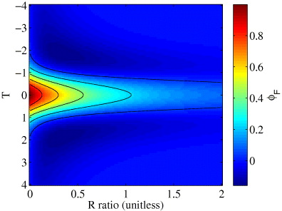
Figure 2. The effects of frequency filtering a simple flow on the correlation function. The amplitude of the correlation function decays rapidly as R increases.
Download figure:
Standard image High-resolution imageThe amplitude of the correlation function decays rapidly as R increases and the effects on the shape of the function are quite minimal (figure 2). The correlation function can still be approximated by a Gaussian. Moreover, the error on the fitted width is not very important in STICS as we are interested in finding the peak centroid at each time lag.
The same development still holds for a diffusing population, but the calculations are more complicated due to the shape of equation (15). For the sake of brevity, we will simply state the result for the amplitude of the filtered 2D diffusion correlation function, ϕF,d(0).

where we used a definition of the exponential integral,  and defined another dimensionless ratio, S = 2πνcw2r/4D. A flowing population and a diffusing one sharing a similar time scale (4Dw2r = v/wr) will be filtered similarly (not shown).
2.6. Symmetry filtering
A simple alternative to filtering is to use the fact that the only time asymmetric component in the correlation function is the flow. Effectively, a diffusing and/or immobile population behaves the same way backwards in time, as opposed to the flow that will move in the opposite direction. Therefore, one could define an asymmetric correlation function:

This is equivalent to removing the correlation of the time reversed intensity. It is a simple way to isolate the flow without disturbing it. However, the correlation function is still computed with all the other populations, which can give a noisy asymmetric correlation if the other populations are dominant. Furthermore, photobleaching and other non-stationary effects will be enhanced and should be corrected by 'detrending'.
3. Materials and methods
3.1. Computer simulations
In order to test the techniques developed, computer simulations were run using the custom Matlab (The MathWorks, Natick, MA) routine previously described [18]. These simulations model key aspects of fluorescence microscopy image time series acquisition. A list of typical simulation parameters is found in table 1.
Table 1. List of variable parameters in the simulator along with their typical values. Parameters that were kept constant for data in this paper are indicated in bold.
| Symbol | Description | Typical value |
|---|---|---|
| Δx | Pixel size | 0.2 μm |
| wr | e−2 beam radius | 0.4 μm |
| Δt | Time between images | 2 s |
| T | Number of images in the time series | 120 frames |
| ρ | Particle density | 20 part μm−2 |
| v | Particle velocity | 2 μm min−1 |
| D | Particle diffusion coefficient | 0.01 μm2 s−1 |
| L | Image ROI size | 32×32 pixel2 |
| WF | Width factor of the analogue detection noise | 10 |
Unless otherwise noted, these parameters were used for all simulations. Those that were kept constant for all simulations presented in this paper are indicated in bold. Note that we chose the parameters to closely match what we usually have in real cellular imaging data (i.e. [5]). For each data point shown, 32 simulations were run and the results are indicated either as mean ± standard deviation (STD) or as boxplots. The focus was on accuracy rather than precision since we analysed small regions of interest (ROI) and typically many of these can be fit inside a single cell. Dashed lines were included in the graphs to indicate the acceptable region where the relative error is less than 20%, which is less than the typical broad biological distribution encountered with small finite populations of cells.
3.2. Data analysis
For the IIR filtering, a highpass Butterworth filter was converted numerically through bilinear transformation. The data were then filtered pixel by pixel. The correlation function was computed and we rejected long time lags where the maximum of the function was of similar amplitude to random fluctuations. A Gaussian was fit for each time lag, and the slope of a linear fit of their centroid positions was used to determine the velocity. To extract the flow density, we used a linear regression on the fitted volume (height times BA) to obtain the zero lag peak height (as the correlation at τ = 0 will contain other components). This amplitude was normalized by the total amplitude obtained with ICS, to obtain a flow fraction. For biased diffusion, we did a nonlinear fit of the peak amplitudes with equation (18).
For the asymmetric analysis, we subtracted the space–time correlation function of the time-reversed data from the normal one. This created a negative peak in the direction of the flow. We then fitted two Gaussians of equal but opposite positions and amplitudes for each time lag. We rejected the first lags where the two peaks were too close to be distinguished and used the same criterion as in IIR filtering to reject the long lags. We then proceeded similarly to the IIR filter to obtain the flow velocity and density. For the diffusion coefficient, we used the slope on the linear fit of the peak width according to equation (18).
For the nICS analysis, we use a Hamming window half the time length of the signal. We then averaged the nICS correlation function obtained for three half-overlapping time windows. A nonlinear regression of the whole correlation function with equation (28) was used to extract the velocity. This equation was convolved in frequencies with the Fourier transform of the autocorrelation of the window. The peak amplitude was normalized to the total ICS peak amplitude to extract the flow fraction. For biased diffusion analysis, we fitted the time-Fourier transform of (18) (windowed by the autocorrelation of the Hamming window) to extract the different fit parameters.
Simulations including photobleaching were 'detrended' as specified in the following references [14, 15]. Briefly, the mean intensity of the images in the time series was fit to a mono-exponential decay. Random numbers were added to each pixel so that the average intensity would stay constant over time.
3.3. Cell culture and plasmids
CHO.B2 cells (from Rudi Juliano and co-workers [19]) were cultured in DMEM medium (Invitrogen). Cells were transfected with Lipofectamine and Lipofectamine 2000 (Invitrogen) according to the manufacturer's instructions and α6-GFP and mCherry-paxillin were expressed as previously described [5, 20]. αL-GFP and β2-GFP were made by in-frame replacement in αL-YFP and β2-YFP, kind gifts of T. Springer.
3.4. Total internal reflection fluorescence (TIRF) microscopy
Image time series were acquired on an Olympus IX70 inverted microscope (1.45 NA oil 60 × PlanApo objective) with a Ludl modular automation controller (Ludl Electronics Products) controlled by Metamorph (Molecular Devices). The 488 nm laser line of an argon ion laser and the 543 nm laser line of helium–neon laser (Melles Griot) were used to excite GFP and mCherry, respectively, and a dual emission filter (z488/543) was used to separate emissions. Images were acquired via a charge-coupled device camera (Retiga Exi, Qimaging).
The laminin (LM) and ICAM ligands were adsorbed to coverslips pre-coated with 1 mg ml−1 poly-l-lysine, which has been previously reported to improve adsorbtion [21, 22].
4. Characterization in silico
4.1. Frequency filtering
To verify the theory of the frequency filter (equations (30) and (31)), we simulated simple flows and diffusion while changing the characteristic dimensionless ratio. We changed R/S by varying one parameter and keeping the other constant (νc = 2.5 mHz, v = 2 μm min−1 / D = 0.01 μm2 s−1 and wr = 0.4μm) and computed the remaining fraction of molecules by ICS. The results, shown in figure 3, agree well with the theoretical function, except for a general higher bias. This bias is probably due to the fact that we are still fitting a Gaussian to the correlation function. Therefore, the two negative sidelobes (as seen in figure 2) create an apparent greater 'Gaussian amplitude'.
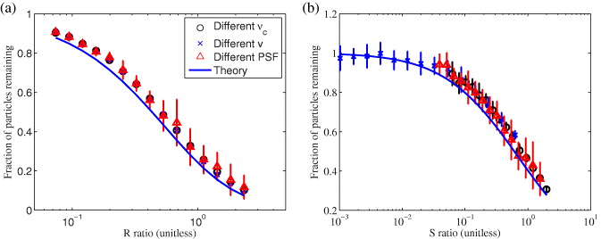
Figure 3. Fraction of particles remaining after applying a Butterworth filter on a flowing (a) / diffusing (b) population as a function of R/S. This ratio was changed by varying one of the three parameters (νc = 2.5 mHz, v = 2 μm min−1/ D = 0.01 μm2 s−1 and wr = 0.4 μm). The effects of filtering a population depends only on the dimensionless variable and agrees well with the theoretical equation. The higher bias for the experimental values is caused by the Gaussian fitting, where the negative sidelobes create an higher apparent 'Gaussian amplitude'. Data are expressed as mean ± STD.
Download figure:
Standard image High-resolution image4.2. Comparison of new techniques
4.2.1. Pure flow
We extracted the fraction of molecules flowing (f), the recovered velocity (v) and angle (θ) as a function of increasing numbers of immobile particles and noise (width factor of the analogue detection noise (WF)). As correlation techniques are generally not affected by white noise (except in the zero lag), we added correlated noise in the form of a fast diffusion on the time scale of analysis (D = 1 μm2 s−1). In this analysis, we identified the fraction of mobile particles and split the rest equally between immobile and diffusing particles. Unless otherwise noted, default simulation parameters were used (see table 1).
We simulated an immobile fraction of up to 90%, a WF of up to 20 (where the SNR is approximately one) and a mobile fraction down to 10%. In most of these difficult situations, the techniques did not show a significant decrease in accuracy or precision (figure B.1). This suggests that the new techniques are not greatly affected by these parameters. Note that the accuracy of all techniques is not very good for recovering the fraction of molecules flowing as it relies on ICS and this technique works poorly in these low sampling conditions (small ROIs [18]).
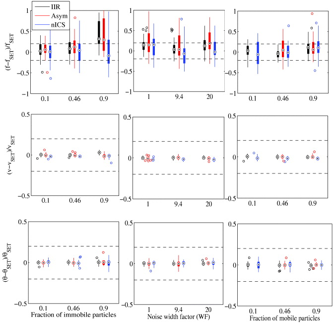
Figure B.1. Accuracy and precision comparison of IIR, the asymmetric analysis and nICS for measuring simple flow. Statistics calculated from 32 simulations each with image series of 32 × 32 pixels by 120 frames. Boxplots as in figure 4.
Download figure:
Standard image High-resolution image4.2.2. Biased diffusion
One can think of biased diffusion (simultaneous diffusion and flow) as a more realistic model of directed molecular transport in a cell. Effectively, due to the stochastic nature at the molecular level in the low Reynolds number sub-cellular environment, biological transport is probably never perfect flow. We define here a transport bias coefficient, B = vwr/4D, so that it is close to one when flow and diffusion are on the same time scale.
We compared the new techniques as a function of the transport bias coefficient (figure 4). For the fitted density, the IIR analysis is accurate over most of the range. For nICS, it becomes heavily biased upwards as the fit fails more frequently, converging to a null velocity and a very high density. The asymmetric analysis gets slowly biased towards zero. As for the velocities, all of the techniques start diverging at a ratio of around 0.6.
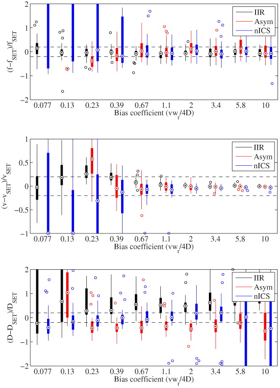
Figure 4. Accuracy and precision comparison of IIR, the asymmetric analysis and nICS for measuring biased diffusion. Statistics calculated from 32 simulations each with image series of 32 × 32 pixels by 120 frames. Targets indicate median, the edges of the box the 25th and 75th percentiles and the whiskers extend to the minimum and maximum value excluding outliers (more than 1.5 times the length of the box away from the median).
Download figure:
Standard image High-resolution imageWe were also able to fit the diffusion coefficient of the flow, which provides more information about the biological process. For the IIR and asymmetric analysis, the fit is very approximate and only the order of magnitude estimate of the diffusion coefficient could be obtained for a B between 0.2 and 5. The two techniques have an opposite and similar bias. Effectively, we used different methods in the IIR and asymmetric analysis to extract the diffusion coefficient. nICS performs remarkably well as it is able to measure an accurate and precise diffusion coefficient down to a bias coefficient of 0.2, even if it fails to fit the velocity and density. At high bias coefficient, the relative error becomes large since the diffusion coefficient is very low.
We repeated all the simulations for a biased diffusion; setting D to 0.005 μm2 s−1 to obtain a B close to one (figure B.2). The techniques are generally less precise than for pure flow, but display acceptable accuracy over a wide range of parameters.
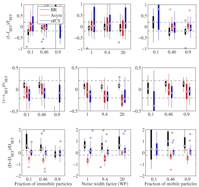
Figure B.2. Accuracy and precision comparison of IIR, the asymmetric analysis and nICS for measuring biased diffusion (B = 1). Statistics calculated from 32 simulations each with image series of 32 × 32 pixels by 120 frames. Boxplots as in figure 4.
Download figure:
Standard image High-resolution imageIt is important to note that the IIR filter shows a higher bias in velocity. For a biased diffusion, the correlation function will spread as well as move for increasing time lags. This creates an apparent spread in velocities in the direction of the flow. Therefore, the filter will remove more of the low 'apparent velocity' than the fast ones (as it is a highpass). This distorts the correlation function, pushing the centroid of the peak in the direction of the flow and creating a higher measured velocity. In this paper, we carefully chose the cutoff frequency so that the effect would be minimal, but over filtering can lead to velocity up to two to three times higher than the real one (not shown). This effect is not present in the other techniques and highlights the importance of carefully selecting a cutoff frequency for filtering and verifying with other approaches.
We also verified that we could 'detrend' the time series that were affected by photobleaching. The results, shown in figure B.3, demonstrate that the correction was successful at all of the levels tested. The precision of the techniques gets lower as the fraction of bleached molecules increases, however, the accuracy is still acceptable even after 90% of molecules have bleached during the time series, which would be an unacceptable level for most live-cell imaging experiments. It is not very surprising that the techniques are not sensitive to photobleaching, as the correction involves adding uncorrelated random numbers (i.e. noise), and white noise does not significantly affect correlation techniques at non-zero lags.
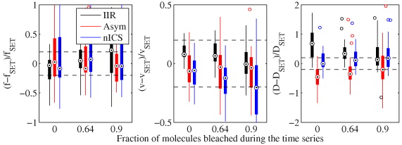
Figure B.3. Accuracy and precision comparison of IIR, the asymmetric analysis and nICS for measuring biased diffusion in the presence of photobleaching. Statistics calculated from 32 simulations each with image series of 32 × 32 pixels by 120 frames. Boxplots as in figure 4.
Download figure:
Standard image High-resolution image5. Characterization in vivo
To test the techniques in living cells, we remeasured the transport properties of proteins we recently studied [5]. We imaged CHO.B2 cells plated on ICAM or LM and transfected with the appropriate integrin (αLβ2 and α6, respectively). Figure 5 shows the results for fluorescently tagged proteins (integrin-GFP and paxillin-mCherry) undergoing retrograde flux in cells plated under these conditions. The asymmetric analysis succeeded sporadically, confirming its higher sensitivity to noise. The velocities obtained with the other techniques are consistent with each other and very similar to what we obtained previously with STICS [5], indicating that the cutoff frequency chosen for the filtering does not significantly bias our analysis. Finally, the diffusion coefficients of the flow are quite high and the transport bias coefficients are very low (near the detection limit of the techniques). It is interesting to note that the fraction of molecules undergoing flow is similar for both types of integrins and lower than that for paxillin. Also, the nICS analysis of the flow fraction is very biased upwards while the asymmetric analysis towards zero, consistent with a low transport bias coefficient.

Figure 5. Molecular transport of α6 and αL integrins and paxillin in transfected CHO.B2 cells. (a) Typical transport map for GFP-αLβ2 integrin and mCherry-paxillin obtained with nICS analysis, where velocity magnitude is indicated by the colour bar. Analysis parameters are 32 × 32 pixel2 regions for 120 frames at 2 s per frame, 0.2146 μm px−1. Vector scale bar is 5 μm min−1 and ROI size is shown by a white square. Summary results of velocity magnitude (b), fraction of flowing molecules (c), diffusion coefficient of flow (d) and transport bias coefficient (e). Black circles represent IIR analysis, red triangle asymmetric analysis and blue cross nICS analysis. Data are expressed as mean ± STD.
Download figure:
Standard image High-resolution image
Taken together, it is clear that the very diffusive flow limits our analysis techniques. The biological process of retrograde flow of adhesion protein is more accurately described by a biased diffusion. More interestingly, the diffusion coefficient of the flow is greater on ICAM than on LM, but the transport bias coefficient also seems slightly higher. A simple model could account for the data; the force generated by the myosin would be proportional to the drag coefficient of the integrins times their velocity, but the diffusion would only depend on the drag coefficient. This suggests that the interaction between integrins and their respective ligand is different (drag coefficient), but also that the total force exerted by the myosin is different. Previously, we performed centrifugation assays [5] to verify that the interaction between integrins and their ligands was indeed different, but could not determine if feedback loops had an influence on the force.
6. Discussion and conclusion
We established a generalized theoretical framework for ICS that serves as a basis for connecting and comparing variants of these methods. It also provides an easy way to extend the correlation techniques to more complicated dynamics as well as a better understanding of the sources of error. We developed, characterized and tested three new tools to measure molecular transport. STICS with the IIR filter emerged as a robust technique to measure molecular flow velocities in single cells, densities and transport bias coefficients. Filtering is however limited by the transport bias coefficient; over filtering can lead to biased velocities. We developed expressions for nICS for the cases of a pure flow, diffusion and biased diffusion and it is a promising new space for unbiased transport measurement without requiring filtering. It complements STICS and is of crucial importance in determining a proper cutoff frequency for the IIR filter. It also provides an excellent estimate of the diffusion coefficient of the flow over a wide range of parameters. The asymmetric analysis was more noise-sensitive; however, it can provide accurate measurements in high signal-to-noise data sets.
These techniques allowed measurement of two new molecular transport parameters: the protein density and transport bias coefficient in single cell. Computer simulations showed that the main limitation of the techniques was the diffusive property of the flow. We demonstrated that molecular flow, at least in this biological system, has a significant diffusive component. A better representation of molecular transport is diffusion biased in one direction. This can be deduced from first principles but was not previously shown. Further improvement of the techniques could shed light on intricate biological processes such as cell migration that depend in part on protein transport, by effectively resolving different contributions to molecular transport, such as force and drag coefficient.
Acknowledgments
PWW acknowledges funding support from the Natural Sciences and Engineering Council of Canada (NSERC) and the Canadian Institutes of Health Research (CIHR). LPT acknowledges fellowship support from Fonds québécois de la recherche sur la nature et les technologies (FQRNT) and NSERC. ARH was supported by National Institutes of Health grants GM23244 and the Cell Migration Consortium (U54 GM064346).
Appendix A.: Derivation of the effects of the infinite impulse response filter
For a flowing population with a Gaussian PSF, the intensity in one pixel is:

where wr is the e−2 radius of the PSF and xi(t) = x0 + vt is the position of particle i at time t. Therefore, the (mean-corrected) correlation function is:

In general, if we filter the intensity beforehand, denoting F(t) the output of the filter h(t):
In other words, the correlation function of the output of the filter, ϕF(τ), is convolved with the autocorrelation of the filter impulse response. The power spectrum of F(t) is then

The correlation function is filtered by the absolute value squared of the frequency response of the filter. This is why we do not need to care about the phase response of the filter. We will consider here the lowpass first-order Butterworth filter to find the shape of the filtered intensity. In that case, the frequency response has the shape of a Lorentzian function

where νc is the cutoff frequency of the filter. The filtered correlation function will be convolved by the Fourier transform of (A.5), which is the double-sided exponential decay. Computing the convolution integral, we have
Introducing two dimensionless variables, a R = πwrνc/v ratio and a normalized time T = tv/wr, this simplifies to
