


Abstract
We present a fully quantum mechanical treatment of collisional correlations beyond mean-field dynamics. Correlations are handled by an ensemble of mean-field states emerging from a stochastic propagation scheme. This is done by first propagating two-body correlations in time-dependent perturbation theory for a certain time span, reducing the coherently correlated state into an incoherent sum of two-particle-two-hole states, and then sampling this state into an ensemble of mean-field states according to the jump probability obtained from perturbation theory. The scheme is applied to a simple 1D test case calibrated to typical scales of molecules and clusters. Even for the small system size and low dimension, the scheme produces robust results. Occupation numbers and entropy show steady relaxation towards thermal equilibrium.
Export citation and abstract BibTeX RIS

Content from this work may be used under the terms of the Creative Commons Attribution 3.0 licence. Any further distribution of this work must maintain attribution to the author(s) and the title of the work, journal citation and DOI.
1. Introduction
We propose a stochastic, microscopic description of non-equilibrium quantum dynamics in finite many-fermion systems accounting for collisional correlations. The theory is designed for the regime of high excitation where coherence at the two-body level is unimportant due to the large phase space involved. Typical such processes are induced nuclear fission and low-energy nuclear collisions [1, 2], excitation of molecules and clusters by intense laser pulses [3], ballistic electron transport in nano-systems [4], or thermalization in trapped Fermi gases [5]. The notion 'collisional correlations' is taken from Fermi liquid theory [6] where two-body correlations are reduced incoherently to two-Fermion collisions. Non-equilibrium dynamics at the level of Fermi liquid theory was since long successfully applied to several bulk systems. More involved is the detailed modeling of non-equilibrium dynamics in finite Fermion systems, required, e.g., for irradiation of molecules and nanosystems. Fast development of lasers and imaging techniques [3, 7] indeed promises to reveal soon time resolved details on non-equilibrium dynamics, which is, for example, crucial for understanding, and ultimately controlling nano systems by light.
The prototype model of non-equilibrium dynamics is the Boltzmann equation which allows to describe and understand microscopically thermalization in classical many-body systems in terms of two-body collisions. The Boltzmann equation has been applied with success to a wide variety of classical systems [8]. There exist also extensions to account for dynamical fluctuations, e.g., by a Langevin term [9, 10]. More involved is the description of many-fermion systems. Two new features need to be taken care of, the Pauli principle which prevents collisions into occupied states and the uncertainty principle which inhibits a local treatment of collisions (as used in the Boltzmann equation). The resulting quantum kinetic equations become highly involved and hardly applicable in realistic finite systems [6, 11]. Practically, the Pauli principle can be accounted for by extending the Boltzmann equation to the Boltzmann–Uehling–Uhlenbeck (BUU) form [12]. It then provides a pertinent description of fermion systems where quantum shell effects can be ignored. These are homogeneous fermion liquids (gases) as electrons in solids [4] or nucleons in a neutron star [13]. Furthermore, BUU can be considered as a semi-classical treatment, thus applicable to finite fermion systems, but only when sufficiently large excitation energies, or temperatures respectively, allow to ignore quantum shell effects. It has been widely used this way for describing nuclear reactions [14, 15], laser excitation of metal clusters [3, 16, 17], or electron transport in wires [18]. Particularly in the nuclear context there also exist some examples of extensions to include fluctuations, augmenting BUU by a Langevin term [2, 19–21].
In electronic systems, recent attempts aim at treating correlations at semi classical level on top of quantum mean field [22] in the line of Time Dependent Density Matrix approaches [23]. There also exist some investigations based on Time Dependent Current Density Functional Theory (DFT) which allows to account for some dissipative behaviors but the approach is not directly suited to finite systems as it fails to provide total energy conservation, at least in its present formulations [24, 25]. Fully quantum mechanical treatments remain rare. There are, e.g., some studies in schematic model systems [26] and, more practically, in the time-dependent configuration-interaction method [27]. However, these very elaborate treatments are still restricted to very small systems and/or low excitations. In spite of its urgent need, a practical, robust quantum dynamical theory of collisional correlations in the regime of high excitations in nuclei, molecules and nano-particles thus does not yet exist. We propose here a formal and practical route to develop such a theory which will then serve as an extension of the well established collision terms in semi-classical BUU to the quantum mechanical regime. Our approach is generic and applicable to any finite fermion system where two-fermion collisions play a role in the dynamical evolution. As a first test, we consider here a simple illustrative test example in 1D. The approach proposed here relies on an early formal investigation [28] formulated in terms of density matrices. It is reformulated here on a wave function basis and within restricting incoherent correlations to leading order. It is then applied to an illustrative example to demonstrate its capabilities.
2. Formal framework
2.1. Stochastic TDHF reformulated
Our formal starting point is Stochastic Time-Dependent Hartree–Fock (STDHF) [28], which provides a description of dynamical correlations in terms of a stochastic ensemble of TDHF (mean-field) states. Although originally formulated in nuclear dynamics, it can be used in any system where a quantum mean field provides a sound description of ground state and low-energy properties, such as nuclei, molecules, or clusters. In the electronic case the underlying practical framework will be DFT [29] with local density approximation (LDA) as associated effective mean field. Time dependent LDA (TDLDA) is meanwhile widely used for simulating various dynamical scenarios [30, 31]. STDHF as proposed here is equally applicable to DFT thus delivering a Stochastic TDLDA (STDLDA).
Originally, STDHF was formulated in terms of density matrices with the von Neumann equation as formal starting point. It was also shown that STDHF can be reduced to a quantum Boltzmann–Langevin equation, namely a kinetic equation for the one-body density matrix containing a stochastic term beyond standard kinetic picture [28]. STDHF thus formally contains all ingredients for describing the path to thermalization and the thermal fluctuations around it [2, 28]. But it has never been explored in practice at full quantum level because of its complexity. Our aim here is to reformulate the theory in simpler terms, restricting correlations to their leading two-particle-two-hole ( ) contribution.
Means of the description is an ensemble of  Slater states
  . The
. The  are built from single-particle (s.p.) states
  , where
  stands for the occupied (hole) states. We also carry a sufficient amount of unoccupied (particle) states
  to supply space for the stochastic jumps to come. The enlarged space now allows to unfold the hierarchy of n-particle-n-hole (nph) excitations. The
  excitations need not to be taken care of, as they are already accounted for in the mean-field ground state and propagation. The first true excitations beyond mean field come along with
  states

which as such are, again, Slater states. The idea is then to propagate for some time a correlated state  starting from an uncorrelated situation,
  . After a certain propagation time τ this coherent state
  is sampled in terms of an ensemble of pure Slater states
  , where
  and
and  is the probability with which
  appear. The weight of the original state
  is the complement
  (we attribute
  to the 'no transition' case).
We evaluate  in first order time-dependent many-body perturbation theory, propagated over a time span τ and delivering eventually the transition probability according to Fermiʼs golden rule [28]. In the
  picture it reads in detail


where  is the residual interaction complementing the mean-field Hamiltonian
  . The rearrangement energy
  corrects for the change in the mean field due to the actual
  transition (the actual transition preserving the total energy by construction [28]). It is negligible in large systems because 2 changing states out of hundredth of particles will not matter much. However, it cannot be ignored in small systems we want to address. The ϑ in equation (2) is the Heaviside function. The finite width is realistic as it can be related to a finite sampling time and, even for long sampling times, to the fluctuations of the s.p. energies in a mean-field (TDHF/TDLDA) evolution. The Heaviside function is used because it is technically the simplest finite-width function. Moreover, we are not trying to adjust the width to propagation time τ. In this first (proof of principle) paper, we simply employ the width
  as a numerical parameter to deal with collisions in a discrete spectrum. Of course, the width spoils to some extent energy conservation. One has thus to find a good compromise for
  . It has to be larger than the average distance of excitation levels to provide an appropriate coverage of reaction rates. On the other hand, a small
  is preferable for minimal violation of energy conservation.
Note that the scheme is based on time-dependent perturbation theory. It thus stays in the weak coupling limit typical of standard kinetic theory. This implies restrictions on the strength of the residual interaction  and on the choice of the sampling interval τ [28, 32]. The restriction on the amplitude of
  is governed by the nature of the considered system. As long as mean field provides a good starting point,
  is expected to be small enough. The restriction on τ is more of practical nature. Indeed τ has to be long enough to randomize the quantum phase oscillations in the
  correlations, thus justifying stochastic reductions and loss of coherence, but short enough to maintain
  . This means that in practice it has to be checked that it fulfills the above conditions. Once fixed it then allows to preserve perturbation theory on short time (of order τ) while allowing the progressive building up of (possibly large) perturbations (well beyond the pertubative regime) on long times (
 ).
).
2.2. Stochastic ensemble description of the dynamics
The stepping scheme thus proceeds as follows. An initial state  is defined and each member of the ensemble is initially set to
  . Each
  is then propagated individually. First, we propagate from 0 to τ by TDHF/TDLDA. At time τ one scans all
  states about
  and evaluates the jump probabilities
  according to equation (3). One state
  out of the possible κ is then chosen randomly according to its weight
  . Subsequently, we propagate
  by TDHF/TDLDA from τ to
  and perform another stochastic sampling at
  and so on. The above procedure is restarted from initial time for each member of the ensemble separately delivering eventually the ensemble
  :
:
The s.p. energies entering crucially the  function in equation (3) require a word of caution. A Slater state
  is invariant under an arbitrary unitary transformation amongst the occupied s.p. states
  . Thus the definition of s.p. energies is ambiguous. But the δ function in equation (3) is, in fact, an approximation. The full expression involves an operator δ function of the mean-field Liouvillean [28]. The replacement by s.p. energies is justified only if the uncertainties on the s.p. energies are small. To minimize these uncertainties, we diagonalize the actual mean-field Hamiltonian amongst the set of occupied states and also amongst the unoccupied states (as we have the freedom to do so) and use the emerging s.p. states and eigenvalues in equation (3). This renders the choice of s.p. energies unique and achieves the best possible approximation to the mean-field Liouvillean.
Once the ensemble  constructed, we can compute any observable by standard statistical averages. One-body observables, in particular, are deduced from the (correlated) one-body density operator built from the total ensemble as

The second representation therein employs the natural s.p. orbitals  . These are the orbitals which diagonalize
  . The eigenvalues are the (fractional) occupation numbers
  of the natural orbitals and provide a natural tool for analyzing thermal effects. A useful quantity deduced from that is the distribution of occupation number
  built from identifying
  (see figures 1 and 2 below). We also use the
  to evaluate the one-body entropy

which characterizes the approach to thermal equilibrium ( is Boltzmann constant).
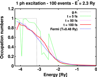
Figure 1. Distribution of occupation numbers  sampled with propagating an ensemble with 100 events after
  excitation with energy
  Ry. Shown are snapshots for a few selected times as indicated. The black, fine dashed line shows the ground state occupation numbers as a guideline.
Download figure:
Standard image High-resolution image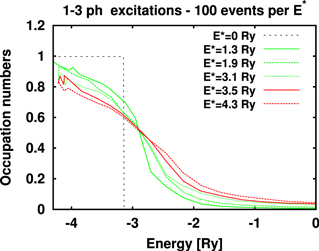
Figure 2. Distribution of occupation numbers  sampled with propagating ensembles with 100 events at final time for
  (green) and nph (red) excitation energies
  . The black, fine dashed line shows the ground state occupation numbers.
Download figure:
Standard image High-resolution imageA word is in order about the level of analysis. Equation (5) defines what is called the one-body entropy, which is the standard entropy associated to a (one-body) mean field description. In a pure TDHF time evolution the occupation numbers  remain strictly 0 or 1, as fixed at initial time, and the entropy strictly 0. Coherent correlations (on top of a mean field description) would lead to some fractional
  , even in the ground state. They would produce pattern which would stay far away from a thermal Fermi distribution and possibly pollute thermal observables. This problem is nevertheless negligible in the present case as we consider high excitations where thermal effects dominate anyway. Thus we think that the definition of entropy and temperature at one-body level suffices for the present purposes and clearly shows how the present theory allows to accommodate the building up of thermal effects, especially as compared to a pure mean field approach.
3. A molecular example
3.1. Outline of the model
For a first exploration and proof of principle, we consider a simple 1D model mimicking a moleculer case with the mean field Hamiltonian (in x representation,  )
)

where  is the local one-body density. For the external potential
  we use a Woods-Saxon profile
  with
with  Ry,
Ry,  a0, a = 2 a0, complemented by a confining harmonic oscillator
  with
with  Ry, acting outside the potential well (
 ) and ensuring soft reflecting boundary conditions. This allows to focus the analysis on thermalization by avoiding competition with ionization. For the self-consistent term we use
  Ry
Ry
 . This model resembles a typical situation in molecules or clusters, where the ionic background provides a spatially fixed external potential. With the chosen parameters we obtain a sufficiently dense spectrum of s.p. energies in spite of the 1D restriction, while producing typical molecular/cluster values of energies and time scales. As residual interaction we choose a simple zero-range force
  with
with  Ry, which leads to realistic relaxation times for the entropy (see below). This choice differs from the mean-field (TDLDA) residual interaction according to the mean field used (which should be
  ). A separate modeling of the residual interaction is legitimate, even necessary, to calibrate the collision rates properly in realistic cases. This is common practice in BUU and it is justified by the observation that the collision term should employ the screened interaction and the mean-field part the interaction before screening [33–35].
The test case has nine physical particles with the same spin. Our working space thus has 9 hole (occupied) levels and an arbitrary number of particle (unoccupied) levels. In practice we used 8 particle states. No significant differences were observed when using 16 or 24 particle states. The distance between s.p. level energies typically varies between 10−4 and 2.5 × 10⁻³ Ry in the range of excitation energies we have explored. In order to fix the optimal width  of
of  we have studied its impact on observables of interest, such as the entropy (equation (5)) as well as the a priori highly
  -sensitive number of collisions and find that they are rather stable up to
  Ry turning to moderate growth above that value. The actual choice of
  is thus not so critical. All values up to
  Ry are acceptable. Very small values of
  require larger samples. Thus we choose
  Ry as the compromise for our present studies.
The period associated to the dominant optical transition lies in the fs range (1.15 fs). The time for propagating two-body correlations in perturbation theory is then chosen as  , following [28]. We found identical results for
  and
and  fs. We follow the dynamics on rather long times, typically 100 fs, which is long enough for thermal relaxation studies and much shorter than Poincaré recurrence time [36]. We propagate ensembles with 100 members.
There are several ways to excite the system. We use here an instantaneous initial random (multi)ph excitation. Looking at s.p. energies as a function of time one observes many level crossings between occupied and unoccupied levels. This gives rise to a sufficient number of  energies matchings according to equation (2) and sufficiently large total probabilities (up some 10ʼs of %), to allow enough transitions into new configurations, while remaining in the weak coupling regime.
The STDHF dynamics is then generated for each member of the ensemble. The energy stays constant during TDHF/TDLDA evolution, but may change a bit in stochastic jumps due to the finite width of the  functions in equation (2). The ensemble thus develops a small energy uncertainty and a negligible trend to growing energy. The energy spread in the ensemble only grows within 100 fs to about 0.05 % (
 = 1.9 Ry) to about 0.3% (
 = 3.1 Ry) of the total energy. A small center-of-mass fluctuation correspondingly appears with an amplitude of order 0.05 to 0.1 a0 around average value 0 which is in the average perfectly preserved (no drift).
3.2. Time evolution of occupation numbers
The relevant one-body observables are extracted from the ensemble averaged one-body density matrix  , see equation (4). Figure 1 shows the distribution of occupation numbers
  at a few selected times for the case of an initial
  excitation delivering
  Ry. The s.p. energies
  are evaluated as the energy expectation values of the natural orbitals (equation (4)) from the (ensemble) Hamiltonian
  (
( is the mean field associated to state
  , (equation (6)). The first snapshot at time 5 fs carries still much of the initial
  pattern. The subsequent snapshots show nicely the steady evolution towards a thermal equilibrium distribution. The finite sampling adds, of course, some fluctuations around the leading monotonic trend. The final snapshot looks already very smooth and resembles the typical Fermi distribution of a thermalized state. We can associate a temperature T to this state by fitting a thermal Fermi distribution to this final
  profile. This yields here
  Ry. The corresponding Fermi function is also indicated on the plot for completeness. Note the gradual convergence of the actual distribution towards the profile, in particular on long times.
3.3. Asymptotic behavior: entropy and temperature
Figure 2 shows the final distributions of occupation numbers for various excitation energies  . Increasingly longer tails develop with increasing
  . All profiles resemble thermal equilibrium distributions, particularly for higher energies. Fits to Fermi distributions deliver the following temperatures:
  Ry,
Ry,  Ry,
Ry,  Ry,
Ry,  Ry and
  Ry.
Ry.
As we are dealing with reflecting boundary conditions the initial excitation energy can be fully converted into thermal energy. It thus makes sense to use it in a purely thermal picture. Figure 3 shows the temperatures deduced from fits of the  to Fermi factors and the final values of the entropies S as a function of the excitation energy. The Fermi gas model provides an analytical estimate for both quantities [37] in the low temperature limit in terms of the level density parameter a:

We have evaluated a for the present model by a direct fit of final S versus initial  (lower panel of figure 3). The corresponding estimates of temperatures are also shown in figure 3 (upper panel). The results agree perfectly for the entropy S. There is some acceptable deviation for the temperature. Mind that the temperature was determined from fit of a Fermi distribution to the occupations
  . The fluctuations in
  due to the finite sampling cause some uncertainties which somewhat degrade the computation of the temperature. The entropy is probably more robust in that respect because it is obtained by summing up over occupation numbers.
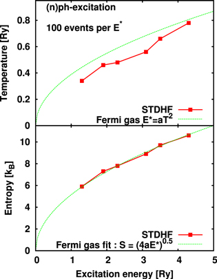
Figure 3. Final entropy (upper) and temperature (lower) as function of excitation energy. The green lines indicate the trends from a semi-classical Fermi gas estimate.
Download figure:
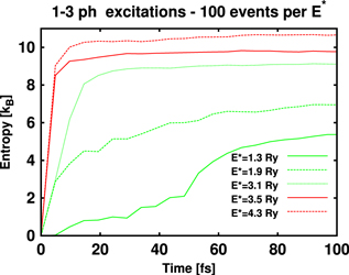
Standard image High-resolution image3.4. Time evolution of entropy and relaxation times
Finally, we extract thermalization time scales from the one-body entropy S, see equation (5). Figure 4 shows the time evolution of entropy for various  . We see the typical pattern of a thermal relaxation process with an early rapid growth turning later to steadily slower increase. Except for the lowest excitation energy probably suffering from too large fluctuations or too low statistics the pattern resemble an exponential relaxation towards the maximum entropy for a given
  . We have fitted exponential relaxation profiles
  to the S(t)ʼs. This delivers relaxation times
  decreasing with increasing
  , from ∼22 fs at
  Ry down to ∼5 fs at
  Ry, representing realistic values for such a system [38].
Figure 4. Time evolution of the s.p. entropy (5) for ensembles of 100 events for  (green) and nph (red) excitation energies
  .
.
Download figure:
Standard image High-resolution image
4. Conclusions and perspectives
We have presented a stochastic approach to include collisional correlations in finite fermion systems. Two-fermion correlations around mean-field trajectories are propagated in first order perturbation theory for a certain time interval. The resulting correlated state is then stochastically reduced to an ensemble of Slater states. One-body observables are computed from the ensemble averaged one-body density matrix. As a proof of principle, we have investigated relaxation processes in a 1D model deducing signatures of thermal equilibration from occupation numbers of s.p. states and associated one-body entropy. We observe clear thermal relaxation processes whose dependence on excitation energy follows nicely the estimates given by a Fermi gas model.
The present results are very promising and call for more investigations and developments. The obvious next step is to gather more experience on the theory from the simple, computationally forgiving 1D model. A typical observable to consider and analyze could be in particular the two-body density matrix as constructed from the ensemble. Extensions to realistic full 3D models are conceivable and will be attacked. These systems have a larger level density and will deliver better statistical averaging properties, but require a much more demanding computational effort. The still too large fluctuations in the regime of low excitation energies require a reformulation of the model in terms of mixed mean-field states. Work along that line is in progress.
Acknowledgments
The authors thank Institut Universitaire de France, Humboldt foundation and European Marie Curie ITN CORINF for support during the realization of this work.