


Abstract
Coupling frequently enhances noise-induced coherence and synchronization in interacting nonlinear systems, but it does so separately. In principle collective stochastic coherence and synchronizability are incompatible phenomena, since strongly synchronized elements behave identically and thus their response to noise is indistinguishable to that of a single element. Therefore one can expect systems that synchronize well to have a poor collective response to noise. Here we show that, in spite of this apparent conflict, a certain coupling architecture is able to reconcile the two properties. Specifically, our results reveal that weighted scale-free networks of diffusively coupled excitable elements exhibit both high synchronizability of their subthreshold dynamics and a good collective response to noise of their pulsed dynamics. This is established by comparing the behavior of this system to that of random, regular, and unweighted scale-free networks. We attribute the optimal response of weighted scale-free networks to a balance between degree heterogeneity, which ensures a good collective response to noise, and the coupling-strength weighting procedure, which overcomes the paradox of heterogeneity that would otherwise impair synchronization.

Content from this work may be used under the terms of the Creative Commons Attribution 3.0 licence. Any further distribution of this work must maintain attribution to the author(s) and the title of the work, journal citation and DOI.
GENERAL SCIENTIFIC SUMMARY Introduction and background. Noise has a regularizing effect in many nonlinear systems. Excitable systems, for instance, pulse with highest regularity for an intermediate noise level, at which random fluctuations 'remind' the system to pulse as soon as the refractory period after a previous spike has ended. This effect is enhanced by coupling to neighbouring elements, but only if synchronization is not too high (otherwise there is no gain from having multiple elements, since all of them behave identically). Thus synchronization and collective noise response seem to be incompatible phenomena. Here we show that a certain coupling architecture is able to optimize the two features simultaneously.
Main results. We study scale-free networks, for which the distribution of node connections follows a power law. Our results show that when the connections in these networks are weighted according to the traffic affecting each link, the system optimizes both synchronizability and noise response, in comparison with unweighted scale-free networks and random networks. This property is attributed to the homogenizing effect of the weighting procedure, which leads to optimal regularity independently of the node connectivity, as shown in the figure.
Wider implications. It is natural to expect that complex systems have either evolved (in the case of living organisms) or been designed (in the case of technological systems), not only to cope, but also to profit, from the inherently high levels of noise existing in nature. We propose a coupling architecture that reconciles collective operation with optimal noise response.
 Figure. Minimum variability in the spiking response of the nodes of three different types of network, as a function of their number of connections.
1. Introduction
In the face of the unavoidable randomness of nature, an appealing hypothesis is that natural systems are optimized to use noise [1]. A particular example of this ability is coherence resonance, also known as stochastic coherence (terms that will both be used interchangeably below), a phenomenon through which noise extracts an intrinsic time scale out of a nonlinear stochastic system, leading to an optimally periodic (coherent) behavior for an intermediate noise level [2–4]. An intuitive understanding of this effect comes from considering a single excitable element subject to noise. Noise excites large-amplitude excursions (such as spikes, or action potentials, in the case of neurons) away from, and back toward an otherwise stable fixed point of the system. These excursions become more frequent for increasing strength of the random perturbations, with the time interval between excursions being bounded from below by a refractory time. At an intermediate noise level spikes pile up and end up occurring almost periodically, at intervals close to the refractory time. For larger noise levels disorder kicks in, degrading that optimally coherent response.
Such a seemingly counter-intuitive constructive role of noise can be further enhanced by coupling in arrays of dynamical elements [5]. Coupling between excitable elements enhances stochastic coherence by 'reminding' a given element in the array to fire when a complying neighbor fires at the 'correct' time (i.e. right after the refractory period has ended). In that way, coherence resonance is enhanced for an intermediate coupling level: when coupling is too small, reminders do not reach the neighboring cells; when it is too large, the array operates almost synchronously, like a single element, and the enhancement effect naturally disappears. The latter effect implies that one can expect strong synchronization to be detrimental to array-enhanced coherence resonance [6].
In the light of the preceding discussion, it would be natural to expect that stochastic coherence is not favored in networks with small-world properties (short path length and high clustering), since such networks seem to favor synchronization [7]. However, it has been observed that the intrinsic heterogeneity of small-world networks, in which different nodes have in general different number of links, leads in fact to a decrement in synchronizability [8], in what has come to be known as the paradox of heterogeneity. Accordingly, stochastic coherence has been shown to persist in small-world networks [9]. Poor synchronizability also occurs in standard scale-free networks, in which the distribution of links reaching a node (its degree) follows a power law, thus leading to substantial heterogeneity among the nodes [10]. This limited capacity for synchronization is concurrent with the existence of multiple instances of noise-induced coherence in these networks [11–13]. Thus synchronization and collective stochastic coherence seem to be incompatible phenomena.
Here we study whether, in spite of the above-mentioned expectations, there are network architectures that exhibit both strong synchronizability and high levels of coherence resonance simultaneously. We concentrate on weighted scale-free networks, in which the strength of the links is scaled according to the local connectivity. These networks have been shown to exhibit large synchronizability [14–16], but is coherence resonance accordingly reduced in them? Our results indicate that this is not the case, and that this coupling architecture, while still supporting a high level of synchronizability, maintains its ability to enhance stochastic coherence through coupling. Thus we suggest that these weighted scale-free topologies are optimal to operate in a stochastic environment when synchronizability is also required.
2. Model
We use a configuration of N excitable elements (which could represent, for instance, neurons) whose dynamics is assumed to be given by the FitzHugh–Nagumo model [2]


where xi is an activator variable and yi an inhibitor variable, i = 1...N labels the neurons, a is a control parameter,  ≪ 1 is the ratio of time scales of the activator and inhibitor, and Ii is a coupling term. The last term in equation (2) corresponds to a white noise of zero mean and amplitude D, uncorrelated between different elements, 〈ξi(t)ξj(t')〉 = 2δijδ(t − t'). In the absence of noise and coupling, the model given by equations (1) and (2) shows a bifurcation to a limit cycle for decreasing a, at |a| = 1. For |a| slightly larger than 1, the system is excitable. The specific values of the parameters used below are a = 1.05 and = 0.01. The equations were integrated using the Heun method [17], which corresponds to a second-order Runge–Kutta algorithm for stochastic equations.
We couple the excitable elements diffusively, representing for instance electrical connections arising at gap junctions between pairs of neurons:

Here g is the coupling strength and nij are the elements of the network connectivity matrix: nij = 0 if i and j are not connected, and nij > 0 if they are connected.
In what follows we consider two main types of network topologies: random Erdös–Renyi (ER) networks, in which the connections are selected at random between pairs of nodes, and random scale-free networks (SFNs) generated with a standard preferential attachment algorithm. In the latter networks, the nodes are connected in such a way that the distribution of degrees (number of connections that a node has with others) follows a power law with exponent γ = 3. This power-law behavior leads to a strong degree heterogeneity among the network elements, which as mentioned above curtails the emergence of synchronization in these networks [8]. The dynamical effects of this structural heterogeneity can be balanced by weighting the coupling strength between each pair or nodes according to the expected (directional) traffic through the edge joining these nodes. A straightforward way to estimate the amount of traffic of a particular edge (i,j) is by means of the edge load ℓij, also known as edge betweenness centrality, which accounts for the traffic of shortest paths that are making use of that link [18]. Specifically, the edge load ℓij is defined as the sum over all pairs of nodes of the network, of the fraction of shortest paths between these that make use of the edge (i,j). This quantity therefore reflects the network structure at a global scale (its value can be strongly influenced by pairs of nodes that may be very far away from nodes i and j). In order to determine the loads of all links in the network, we follow the approach of [15] and count, for each pair of nodes (i',j'), the number n(i',j') of shortest paths connecting them. For each one of such shortest paths, we then add 1/n to the load ℓij of each link forming it. The elements of the connectivity matrix for the weighted SFNs (WSFNs) are then given by

where Ki is the set of neighbors of the ith node. Note that whereas ℓij = ℓji, in general nij ≠ nji. This leads to an asymmetric coupling between any pair of nodes i and j. In ER and unweighted SFNs (UWSFNs), in contrast, nij = 1 for all connected node pairs. In order to do a proper comparison between networks, we rescale the connectivity matrix nij in weighted networks in such a way that , where M is the total amount of edges of the network, as expected in unweighted networks [15].

3. Synchronizability
We first examine the subthreshold dynamics of the excitable elements described by equations (1) and (2). Figure 1(a) shows (in gray lines) the temporal behavior of 11 (out of a total of N = 500) network elements in the absence of spiking activity, for the three different coupling architectures described above: unweighted (UWSFN, top) and weighted (WSFN, middle) SFNs, and random networks (ERN, bottom). The noise intensity (the same for all three network types) is chosen low enough so that spikes are effectively absent. In each case, the average activity of the complete network is shown superimposed to the individual time traces, in thick lines. The amplitude of the fluctuations of that average activity reflects the level of synchronization of the network: a large level of synchronization between the network elements leads to an average activity that resembles that of every single oscillator, which fluctuates due to the added noise. In the absence of synchronization, on the other hand, the dynamics of the different oscillators average out and the fluctuations of the average signal are reduced. Figure 1(a) shows that the average dynamics of the WSFNs (middle plot) fluctuates more strongly than those of the UWSFNs (top) and random networks (bottom), thus suggesting that synchronization of the subthreshold dynamics is stronger in the latter type of network architecture, in accordance with the synchronization properties of that type of coupling topology discussed in section 1 above.

Figure 1. Synchronizability of the subthreshold dynamics of unweighted scale-free networks (black, top plot in panel (a) and triangles in panel (b)), weighted scale-free networks (red, middle plot in panel (a) and circles in panel (b)) and random networks (green, bottom plot in panel (a) and diamonds in panel (a)). Panel (a) shows time traces of selected individual network elements (light-shade lines) and of the average activity of the network (dark-shade lines). Panel (b) shows the synchronization coefficient ρ as a function of the coupling strength g. The parameter values are D = 0.01 and g = 1. Curves in (b) are averages over ten network realizations of each type.
Download figure:
Standard image High-resolution imageIn order to quantify in a systematic way the synchronization capabilities of the three types of networks, we computed a synchronization coefficient as defined in [19]

where the overlines indicate average over nodes, whereas the angle brackets 〈...〉 indicate temporal averages. This coefficient could be read as a the ratio between fluctuations of the global averaged signal and the average of fluctuations of individual network elements. If the system is not synchronized, the individual signals xi(t) will be completely out of step with respect each other and their sum will be averaged out to zero. In the synchronized case, the fluctuations of the global signal are similar to the fluctuations of individual neurons and the coefficient ρ tends to one.
This quantifier is plotted in figure 1(b) as a function of g, showing that all three network types exhibit a smooth transition to synchronization as coupling increases, but the WSFN exhibits a larger synchronization coefficient for all coupling levels, and thus reaches synchronization earlier as coupling increases. A similar enhancement of synchronization is observed in the spiking regime, provided only the subthreshold dynamics is considered (results not shown). Therefore, weighting the connections in an SFN according to expression (4) does lead to a higher synchronizability than standard UWSFNs, and even random networks, in spite of the structural degree heterogeneity of the network.
4. Stochastic coherence
We now turn to the spiking activity of the networks discussed above, and ask whether the increased synchronizability exhibited by the WSFNs concurs with a decreased response to noise of the collective dynamics of the system. Figure 2(a) shows sample time traces of the three networks in the pulsing regime for a fixed noise intensity and coupling strength. In order to quantify in a systematic way the regularity of this spiking dynamics, we analyze the distribution of time intervals between pulses, and in particular we calculate the normalized standard deviation (also known as coefficient of variation) of that distribution, coefficient of variation (CV) , where Ti and σi are the temporal average and standard deviation of those intervals, respectively, for neuron i. The brackets denote the averaging process: we first calculate the CV for each neuron i, averaging in time for 1000 pulses of each unit. Then we take the average over all nodes of the network and finally we calculate the average over the whole set of simulations of equivalent networks (ten for each network type).


Figure 2. (a) Spiking dynamics of the UWSFN (top), WSFN (middle) and random network (bottom) for noise intensity D = 0.5 and coupling strength g = 1. (b) CV versus coupling strength for same noise and the three network types mentioned above.
Download figure:
Standard image High-resolution imageThe dependence of the CV on the coupling strength is seen in figure 2(b). All three network classes show a clear minimum of the coefficient of variation for an intermediate level of coupling strength, which is a signature of array-enhanced coherence resonance [5, 6]: an optimal amount of coupling improves the coherent behavior of the system. Even though the absolute minimum of the CV is of the same order for all three network types, the regularity is larger (the CV is smaller) for the WSFN than for the other two networks for almost all coupling strengths. The difference is specially evident for larger coupling strengths, where the CV is less than half for the WSFNs than for the other two networks. Thus, not only WSFNs synchronize better than the other two complex network architectures, but they also respond better to noise.
Incidentally, figure 2(b) also reveals that the coefficient of variation goes through a maximum for low coupling values in all three architectures. A maximum of the CV versus noise has been reported for low noise intensities in excitable systems that operate close to an oscillatory regime [20]. Given that in array-enhanced coherence resonance the coupling strength effectively controls the noise level, we interpret that the CV maximum observed in figure 2(b) is also due to the proximity to an oscillatory dynamics, which in this case is partly caused by the coupling itself.
In array-enhanced coherence resonance, regular behavior is also enhanced for an optimal noise intensity. This stochastic coherence effect is shown in figure 3, which represents the coefficient of variation versus noise intensity in the three different types of network discussed above, for two values of the coupling strength g. Similarly to the behavior shown with respect to the coupling strength, the CV shows a minimum for an intermediate amount of noise for all three topologies. The minimum CV has a similar value for the three networks in the case of optimal coupling strength, g = 0.1 (figure 3(a)). Additionally, for larger coupling strengths the CV is lowest overall for WSFNs, in particular at the optimal noise level (figure 3(b)). In consequence, we can conclude that WSFNs show both a better synchronizability and a superior collective response to noise.
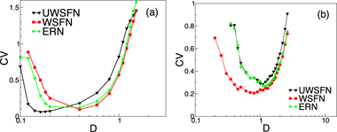
Figure 3. CV as a function of noise amplitude (D) showing stochastic coherence for two fixed values of the coupling strength and for the three networks discussed in the text. (a) g = 0.1, (b) g = 1.
Download figure:
Standard image High-resolution imageWe have not discussed so far how the behavior of the WSFN compares with that of a regular network (i.e. a network with only nearest-neighbor coupling between its elements). Due to the lack of long-range coupling, the synchronizability of regular networks is consistently lower than that of the other networks, as shown in figure 4. Panel (a) in that figure plots the synchronization coefficient defined in section 3 above with respect to noise intensity, for a wide range of noise levels covering both the subthreshold and spiking regimes. The transition between the two regimes can be identified by the sudden increase in ρ occurring at D ∼ 0.1. The figure shows that for almost all noise levels, corresponding to both the subthreshold and spiking regimes, the synchronization is substantially larger for the WSFN than for the regular network. The raster plot in figure 4(b) reveals that the low synchronization of the regular network is due to the finite propagation time of the excitations throughout the network, in comparison with the basically instantaneous propagation enabled by the long-range connections in the WSFN. The raster plot also shows that the regularity of the spike wavefronts is slightly higher for the regular network than for the WSFN since, as mentioned in the introduction, poor synchronization is beneficial for the emergence of array-enhanced coherence resonance. Therefore, taken together, all the results presented so far indicate that WSFNs are superior to all other network architectures considered in optimizing both synchronization and collective noise response simultaneously.

Figure 4. (a) Synchronization level, measured via the synchronization coefficient ρ, versus noise intensity D, for a WSFN (red, circles) and a regular network (blue, squares) and for g = 1. (b) Raster plots showing the location of the pulses in xi for the same two networks with g = 1 and D = 0.5.
Download figure:
Standard image High-resolution image5. Correlating synchronizability and stochastic coherence with degree
In order to investigate the mechanism behind the dual optimality of WSFNs with respect to both synchronizability and collective stochastic coherence, we now examine in detail how these two properties vary in nodes with different degree. First we plot in figure 5(a) the synchronization coefficient ρ for varying node degree k, again comparing the WSFN, UWSFN and random network. This calculation was done following the definition of equation (5), but replacing the average over the whole set of neurons by the average over only the set of neurons with a given degree k. The figure shows that synchronization increases basically monotonically with the degree in all three cases, since higher connected nodes will be more strongly synchronized. However, the dependence of ρ on k is much weaker in the case of the WSFN, which reflects the compensating effect that the coupling strength normalization given by equation (4) has on the coordination between pairs of nodes: when two such coupled nodes have small degrees (which would diminish their synchronization), their connection becomes more important for the global topological structure of the network, thus increasing the coupling strengths between them (and so enhancing synchronization between them). As a consequence, the average synchronization level becomes larger for this type of networks than for unweighted and random networks (figure 1).

Figure 5. Synchronization level at D = 0.1, measured via the synchronization coefficient ρ (a), and minimum value of the CVmin (b), both as a function of the degree node k for the UWSFN (black triangles), WSFN (red circles) and random network (green diamonds) with g = 1.
Download figure:
Standard image High-resolution image
The dependence of the regularity on the node degree is even more revealing. Figure 5(b) shows the minimum (with respect to noise) of the local coefficient of variation for different node degrees. 'Local' here refers to the fact that the CV is computed only for nodes with a given k. This figure shows a clear decrease of CVmin for both UWSFNs and random networks: nodes with low connectivity are substantially less regular than nodes with high connectivity in these networks. In contrast, this behavior is completely absent in WSFNs, where CVmin is basically independent of the degree (and much smaller overall, as noted also in section 4 above). Once again, the coupling strength normalization provided by the weighting of the links balances the disordering effects of having a low degree, thus compensating perfectly the effects of topology heterogeneity, and leading to a homogeneous coherence throughout the network, which results in an enhanced averaged coherence.
6. Discussion and conclusions
Synchronization and collective noise response are in principle opposing phenomena, since array-enhanced coherence resonance requires a certain amount of dynamical heterogeneity: in the limit of perfect synchronization the system behaves as a single unit and coupling would have no effect on noise-induced coherence. Thus it should be expected that systems that synchronize well (such as standard scale-free networks or random networks) have poor collective coherence resonance, whereas systems that do not synchronize perfectly (such as regular networks, in which activity waves propagate spatially with finite speed) can respond positively to noise in terms of their regularity [5]. The results above show that certain weighted scale-free networks exhibit both high synchronizability and a large level of coherence resonance induced by coupling. The weighting process to which the links are subjected in those networks reduces the heterogeneity to a level for which synchronization is now possible, while array-enhanced stochastic coherence is not lost.
The weighting procedure utilized here renders a wide distribution of edge weights similar to that used by Teramae et al [21] in a different setting, namely in networks of synaptically coupled stochastic excitable neurons. That work shows that a combination of recurrence and edge weighting can generate internal noise at a level optimal for spike transmission within the network. Further work is necessary to determine whether a similar mechanism can lead a network to self-organize into a situation in which coherence is optimized by internal noise. Irrespective of the origin of noise, our results allow us to conjecture that the weighted scale-free networks presented here offer an optimal coupling topology for collective operation in stochastic conditions.
Acknowledgments
This work was supported by the Ministerio de Economia y Competividad (Spain, project FIS2012-37655), the Generalitat de Catalunya (project 2009SGR1168), CONICET (PIP:0802/10) and University of Buenos Aires (UBACyT 20020110200314). JGO acknowledges support from the ICREA Academia programme.