


Abstract
We investigate the valley-dependent transport of a graphene system consisting of a uniaxially stretched graphene sheet connected by two unstrained parts, with the interfaces between the strained and unstrained regions along the zigzag direction. A detailed study on the Fabry–Pérot states in the strained region reveals that they carry opposite lateral currents for different valleys when a bias is applied across the interfaces, namely, a pure valley-Hall current arises in the central region. The transverse valley conductance is determined by the number of resonant states in the strained region at the Fermi energy. Like the quantum Hall effect, when Fermi energy is varied, the valley-Hall conductance exhibits step structures and the longitudinal conductance shows peaks.
Export citation and abstract BibTeX RIS

Content from this work may be used under the terms of the Creative Commons Attribution 3.0 licence. Any further distribution of this work must maintain attribution to the author(s) and the title of the work, journal citation and DOI.
1. Introduction
Due to two inequivalent corners K and  of the hexagonal Brillouin zone of graphene, it offers valley degree of freedom similar to electrical charge and spin that can be used to carry information [1, 2]. Electrons of each valley are described by a Dirac equation and cannot be scattered into the other valley by long-range scatterers. The control and detection of the valley index of electrons has drawn much attention in recent years. Valley-dependent physics often arises in graphene systems with line defects [3, 4], spin-orbit coupling [5, 6] or strain. Long and regular line defects are serious challenges in experiments and the spin-orbit effect is often too weak to result in observable effects [1], while, the strain engineering is easily achieved to generate valley dependent physics. Strain exists in a graphene sheet placed on a substrate with different lattice constants [7, 8] and is caused by mechanical stretching in suspended graphene systems [9, 10]. In addition to changing the Fermi velocity [11], strain drifts the Dirac points, which induces opposite effective vector potentials for different valleys [12]. Consequently, localized strain generates a pseudo magnetic field and leads to confined states [13, 14]. The pseudo magnetic field around nano-bulbs and nano-ripples is large enough to be observed experimentally at room temperatures by measuring Landau level spacings [7, 15, 16]. The shape as well as the strain profile of these nano-structures can be engineered and controlled by the substrate morphology and external field [8, 17–19]. A strong and uniform pseudo field is predicted to induce topological insulator states if the Coulomb interaction is taken into account [20, 21]. However, a uniform pseudo magnetic field in a large area cannot be achieved easily in reality because it requires the graphene sheet to be stretched in special ways [22, 23]. Due to the nature of pseudo magnetic fields, a graphene sheet with a strained strip can be used as a device for valley and spin manipulation [24]. It was proposed that a valley current can be pumped by means of periodically changing the strain and other parameters [25–28].
In this paper, we consider the graphene device shown in figure 1, which consists of two unstrained regions and a uniaxially strained central region with the interfaces along the zigzag direction. For an ideal interface with an abrupt change of vector potential for each valley, a huge pseudo magnetic field exists at the interface and has opposite signs for different valleys. Supposing an electron beam is normally incident from the left, the trajectory of electrons with different valleys will be bent by the pseudo magnetic field in the opposite direction at the left interface, forming two Fabry–Pérot states in the strained region, which propagate transversely in the opposite direction, as illustrated in figure 1. Therefore, we expect that a pure transverse valley current arises when a bias is applied across the two interfaces. We analyse the Fabry–Pérot wavefunctions, obtain their density of states between the two interfaces, and find that the lateral conductance for each valley is determined by the number of resonant states at Fermi energy, in addition to a partition factor of electron injection. Our results show that the curve of lateral conductance versus Fermi energy has step-like structures, similar to the quantum Hall effect (QHE). However, the steps of the transverse conductance and the peaks of longitudinal conductance do not align exactly, which is different from QHE. We find that there is an energy window, within which both the lateral and the longitudinal conductances are pinched off. The lateral valley current could be detected by a four-terminal setup with the side arms being placed on ferromagnetic barriers [29, 30].

Figure 1. Sketch of the studied graphene system and the physical origin of the valley dependent transverse transport effect.
Download figure:
Standard image High-resolution image2. Theory and calculations
The graphene system we studied in this paper is shown schematically in figure 1. It has a central strained region of length L sandwiched between two unstrained regions with the interfaces along the y-direction, and the potential in the central region can be tuned by a top gate. In each region, the spinless low-energy Hamiltonians of the electron around valleys K and  in the sublattice basis are
where  is the potential energy profile,
  is the strain-induced vector potential,
  and
and  are the Pauli matrix and wavevector, and
  are the canonical momentums for K and
  valleys. In equation (1) and from there on, we set the reduced Planck constant
  , elementary charge e, and Fermi velocity of graphene
  to be unity for convenience. For both valleys, the eigen energy and the eigen states read

where plus and minus signs correspond to different valleys K and  , respectively. The phase factor appearing in the spinor is defined by

with  being the energy relative to the Dirac point. Since
  and
and  and
and  , we see that
  is the orientation of the velocity of either electron-like or hole-like particles.
The vector potential  is nonzero only in the central region, where its components are given by [31]
  and
and  , in which
  are the components of strain tensor, and
  for graphene [31]. Since the strain is along the x-direction, we have
  ,
,  and
and  . There is also a scalar potential called deform potential
  caused by the strain, which can be absorbed as a part of
  and will not appear from now on. The profiles of the vector-potential and electric potential are described by

Because  is a good quantum number, we assume that an electron of energy E with an eigen wavefunction
  of
of  is injected from the left for valley K. By means of a unitary transform
  defined by
  , we have the following equation

Equation (5) shows that  must be an eigen state of valley
  with the same eigen energy, i.e.,
  . Because the velocity in the y-direction is related to the dispersion by
  , the transverse velocities of these two states are in opposite directions, i.e.,

Therefore, we conclude that under any bias configuration, the transverse currents for two different valleys are the same but in the opposite directions. That is to say, a bias drives a pure transverse valley current in the central region. Of course a longitudinal current also arises, which is non-valley-polarized since the two eigen states have the same x-dependent part. In the following, we will only study the transport of valley K, and the superscripts labeling the valley indices are omitted.
Considering an electron injected from left with wavevector  , transmitting through the first interface and propagating in the central region with the wavevector
  (
( , and
, and  are defined correspondingly), the continuity of the wavefunction at the left interface results in the following equation

where r1 and t1 stand for the reflection and transmission coefficients of the first interface for the left-coming electron. The elastic scattering requires that  and the conservation of lateral momentum
  gives rise to
  . The two coefficients r1 and t1 are found to be

This equation says that there exists a unique incident angle satisfying the relation  , at which the incoming electron of valley K is totally transmitted i.e.,
  , while the electron of the other valley injected at the same angle cannot go through without reflection. This angle is called the Brewster angle in optics, if we make an analogy between the valley polarization and the optical polarization [32]. The transmission and reflection coefficients of the first interface for the right-coming electron can be obtained by exchanging
  and
and  in the expressions of t1 and r1, so we have

Due to the symmetry of the system, the set of transport coefficients of the second interface can be obtained without calculation,

If an electron comes from the left side with lateral wavevector  (or
(or  , in unstrained regions,
  ), it has the probability to penetrate the first interface, bounce back and forth in the central region and propagate laterally. The bouncing state is analogous to the Fabry–Pérot state in optics [33]. It is not difficult to write down its wavefunction by summing over all the right- and left-propagating waves in the central region,
where  is the phase factor acquired by the electron propagating from the first interface to the second interface. Here
  and
and  are defined in equation (2), and represent the right and left propagating states, respectively. To ensure correct propagation directions, the sign of
  should coincide with that of
  . The probability of the electron being found in the central region, namely, the partial density of state in the central region for the left injection, can be obtained by integrating the module square of the wavefunction in the strained region. The calculation detail can be found in the appendix. The left-injected partial state density is

where  is the state density in the center area of both sides injection, and
  is the left-partition factor. They are defined as
The right-injected partial state density can also be obtained as  , where
  is the right-partitioned factor defined by exchanging the positions of
  and r2 in equation (14). The two partition factors satisfy
  to ensure the relation
  .
.
There are interesting features in the spectrum of  on the complex plane of
  . It is easy to see that
  has poles on the complex plane. The poles are defined by the roots of the equation
  . For the electrons that are able to travel through the central region, we must have
  . In this case, the roots are complex numbers. It is not difficult to show that the contour integration
  for each resonant state gives
  in the wide-band approximation (the sign depends on whether the pole is located on the upper half plane or lower half plane), which manifests the property of the density of states. By requiring
  , we have real roots and these real roots correspond to bound states. Figures 2(a) and (e) show the density of states
  as a function of
  and
and  for different V, and figures 3(a) and (e) show
  for different A. In these figures, the bound states are also presented for the purpose of comparison. According to equation (1), relative to the Dirac cone of the unstrained regions, that of the central region is lifted by V vertically and displaced by A horizontally in the
  -
- plane. The resonant states appear in the overlap of the two Dirac cones because real
  and real
  are allowed simultaneously in the area, and the bound states are outside of the overlap region where
  is imaginary. The boundary between resonant states and bound states thus is the Dirac cone of the unstrained regions.
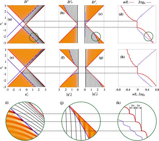
Figure 2. First two rows: contour plots of  (column 1) with the red crossed lines representing the Dirac cone in the strained region and blue crossed lines standing for that of the unstrained regions, contour plots of
  (column 2) and
  (column 3), and the curves of
  and
and  versus
  (column 4) in which we use
  as vertical axis instead of the usually horizontal one in order to align the energy with other subfigures in the same row. The third row: zoom pictures within the circles in the first row. Parameters are
  and
and  for the first row, and the same parameters for the second row except for
  . The units are all dimensionless. They can be restored into the normal units if needed. For example, for the strain
  and the parameter
  eV, the corresponding energy unit and length unit are 0.023 eV and 26 nm, respectively.
Download figure:
Standard image High-resolution image
Figure 3. First two rows: contour plots of  (column 1) with the red crossed lines representing the Dirac cone in the strained region and blue crossed lines standing for that of the unstrained regions, contour plots of
  (column 2) and
  (column 3), and the curves of
  and
and  versus
  (column 4) in which we use
  as the vertical axis in order to align the energy with other subfigures in the same row. Parameters are
  and
and  for the first row, the same for the second row except for
  .
.
Download figure:
Standard image High-resolution image
Under a small longitudinal bias, the nonequilibrium population of the resonant states in the strained region carries the transverse current. The transverse conductance is calculated by  , where
  is the Fermi energy relative to the Dirac point of the strained region, and
  is the transverse current caused by left injection within the energy interval
  through
  .
.  can be obtained from
  in
in  -
- space and the calculation detail is shown in the appendix. When we transform
  into
into  , if the current carried by
  flows upward/downward, we denote it as
  . After a tedious calculation (see the appendix), we have
where  are the numbers of resonant states flowing upward/downward at
  , and
, and  is the net number of resonant states flowing upward. The sign of n determines the transverse current flowing upward or downward. In the calculation, the partition factor
  is treated as a constant, which is 1/2 for our model. One can find that equation (15) has the same form as the Landauer-Büttiker formula if
  is noticed (
 ). The transverse conductance per unit length of the central region (the transverse conductivity) is
  . Though the quantities studied are
  and
and  , we will discuss n instead of
  and
and  themselves.
It is interesting to make a comparison between the transverse conductance and the longitudinal one, which is also related with the resonant states in the central region. According to the Landauer-Büttiker formula, the longitudinal conductivity is

where  is the Fermi energy relative to the neutral point of the unstrained regions, and
  is the transmission coefficient across the central region.
The bound states in the strained region are not involved in the above calculations, because they cannot be populated by the left or right electron injection, and thus cannot cause a Hall-like effect under the longitudinal bias. However, the bound states have their own fantasy properties. Because electrons carried by these bound states cannot escape away into the left and right ends, the strained region serves as an electron wave guide when the strained region is biased laterally [34]. This non-Hall effect is not our aim and will not be discussed.
3. Results and discussions
The profiles of  and
and  , and the curves of n and
  , can be found in figures 2 and 3 for a variety of parameters.
  and
and  behave like stripes in the allowed region of resonant states. The bound states are represented by black lines in these figures. These resonant stripes and bound state lines are almost vertical, and the spacing between two adjacent stripes or bound state lines is about
  , as that in an infinite potential well.
When the Dirac point of the unstrained regions lies outside of the Dirac cone of the central region, i.e.,  , there is an energy window in which no resonant state exists in
  and
and  , and both
  and
and  as well as
  vanish, as shown in figure 2. The curve of n shows step-like structures and the curve of
  manifests peaks. This is quite similar to the quantum Hall effect but without exact step-peak alignment. The steps of n can be understood as follows. Suppose the Fermi energy lies initially within the energy window and then moves downward slowly, every time the Fermi energy passes the joint point between a bound state line and the resonant-bound boundary, a new resonant state participates in the lateral transport, and a step
  appears in the curve of n, as shown in figure 2(i) through (k).
When increasing V, the Dirac point of the unstrained region moves down with respect to that of the central region, and the energy window is therefore shifted downward, as shown in the second row 2 in figure 2. The resonant area above the energy window enlarges while that beneath the energy window shrinks, and resonant areas in  and
and  are modified correspondingly, which leads to the curve of n evolving into an asymmetric one with the step-like structures preserved very well.
Now we change the parameters V and A so as to  . In this case, the Dirac point of the unstrained region lies in the lower part of the Dirac cone of the central region, as shown in figure 3. The energy window where no resonant state exists disappears. Because the upper part of the Dirac cone of the central region is completely filled by resonant area, the resonant states moving upward and those moving downward are almost canceled by each other, i.e.,
  and
and  for
for  . If we draw a horizontal line in plots of
  and
and  to represent the Fermi energy, for
  the line intersects with both the resonant-bound boundary line in
  and that in
  . When the horizontal line moves vertically, sometimes it crosses a joint point on the boundary line in
  , which gives a positive contribution to n, sometimes crosses a joint point in
  , that leads to a negative contribution. This causes the irregularity of the curve of n. When we fix V while decreasing A to zero, the Dirac point of the unstrained region moves horizontally to the vertical axis,
  and
and  are completely symmetric, and n vanishes. During the change of A, regardless of what happens to n, the curve of
  is almost unchanged, because
  is related to the summation of
  and
and  , not the difference between them.
Finally, we briefly comment on what happens when the interfaces are deviated from the zigzag direction by the angle  . According to [25], the vector potential components for this case are
  and
and  . The vector potential is of
  periodic in
  , which reflects the trigonal symmetry of the honeycomb lattice. The overlap between Dirac cones of the strained and unstrained regions is governed by
  , that dominates the main features of the Hall-like transport effect.
  affects the resonant condition, leads to a small deformation of the resonant strips in the contour plots of
  ,
,  and
and  in figures 2 and 3, and only has a minor effect on the detail of the curves of n and
  . The Hall-like transport effect is most apparent for the interfaces along the zigzag direction (
 ), and vanishes along the armchair direction (
 ).
).
4. Summary
We considered the transverse transport of a graphene device consisting of two unstrained regions and a uniaxially strained central region with the interfaces along the zigzag direction under the bias across the central region. A pure valley Hall current arises and is determined by the number of resonant states in the strained area and an injection factor. The longitudinal conductance is also discussed for the purpose of comparison.
Acknowledgments
This work was supported by NSF of China grant nos. 11274124 and 11374246, University Grant Council (contract no. AoE/P-04/08) and Research Grant Council (HKU 705212P) of the Government of HKSAR.
Appendix A.: Derivation of equation (12)
Inserting the expressions of eigen states into equation (11), we have the Fabry–Pérot wavefunction

In equation (A.1), we omitted the y-dependent part because it is irrelevant to our calculation. The left-injected partial density of states in the center region is
In the calculation, we have neglected an interference term between the forward and the backward propagating states since it is much smaller than the dominant term and does not increase with L. At a given  (or a given
  ), taking derivative on both sides of the energy conservation law
  , keeping in mind that
  and
and  , we have
  . Within the interval from
  through
  , the number of states is found to be

where  is understood as the partial density of states in
  -space. It reads
where the relations  (note that the transmission probability of the first interface is
  , not
, not  ) and
) and  have been used. The partial density of states due to the right-injection,
  , can be obtained by exchanging
  and r2 in equation (A.4)
The total density of states corresponding to both sides injection thus is
Combining equation (A.6) and the definition of  in equation (14), we have equation (12).
Appendix B.: Derivation of equation (15)
Now we calculate the lateral current caused by left side electron injection. In the area  in
in  -space, the number of states is
  . Every left-injected state has the probability of
  found in the central region, and thus carries a transverse particle current
  . Replacing
  with
with  in the expression of dS and recalling
  , the transverse current carried by these states is found to be
Because  is the orientation angle of the velocity in the central region, two parts of the integration indeed correspond to up-flowing and down-flowing current respectively.
  can be rewriten as
  for
for  and
and  for
for  . The integration over
  can be converted into that over
  by using the relation
  , which is derived from equation (3) at fixed
  . As mentioned below equation (11),
  has the same sign as
  , so we have
  . This transverse current is finally given by
The transverse conductance due to an electron coming from the left is
We have equation (15).