


Abstract
The objective of this study is to investigate under what circumstances Förster theory of electronic (resonance) energy transfer breaks down in molecular aggregates. This is achieved by simulating the dynamics of exciton diffusion, on the femtosecond timescale, in molecular aggregates using the Liouville–von Neumann equation of motion. Specifically the focus of this work is the investigation of both spatial and temporal deviations between exciton dynamics driven by electronic couplings calculated from Förster theory and those calculated from quantum electrodynamics. The quantum electrodynamics (QED) derived couplings contain medium- and far-zone terms that do not exist in Förster theory. The results of the simulations indicate that Förster coupling is valid when the dipole centres are within a few nanometres of one another. However, as the distance between the dipole centres increases from 2 nm to 10 nm, the intermediate- and far-zone coupling terms play non-negligible roles and Förster theory begins to break down. Interestingly, the simulations illustrate how contributions to the exciton dynamics from the intermediate- and far-zone coupling terms of QED are quickly washed-out by the near-zone mechanism of Förster theory for lattices comprising closely packed molecules. On the other hand, in the case of sparsely packed arrays, the exciton dynamics resulting from the different theories diverge within the 100 fs lifetime of the trajectories. These results could have implications for the application of spectroscopic ruler techniques as well as design principles relating to energy harvesting materials.
Export citation and abstract BibTeX RIS

Content from this work may be used under the terms of the Creative Commons Attribution 3.0 licence. Any further distribution of this work must maintain attribution to the author(s) and the title of the work, journal citation and DOI.
1. Introduction
Excitation (or electronic) energy transfer (EET), also sometimes referred to as resonance energy transfer, is an important process exploited throughout nature. It involves the transfer of energy from an initially electronically excited species such as an atom, molecule or chromophore (the excited state donor) to another nearby species in the ground electronic state (the excited state acceptor). When the donor returns to its ground state, the acceptor becomes excited. Fundamentally this is a quantum mechanical process that involves the exchange of a virtual photon between (valence) electrons of the two species. Electronic energy transfer can be highly efficient, as exemplified by many natural photosynthetic organisms whereby solar energy is captured by their antenna complexes and transferred to their reaction centres, often with over 90% efficiency [1, 2]. Due to the importance of EET in the development of solar energy harvesting technologies, it is not surprising that enormous effort has been undertaken to understand the mechanisms behind such efficient photochemical systems [3–6]. This has resulted in a wide range of synthetic structures that are able to mimic some features of natural antenna complexes [7–10]. Further to this, a great deal work has been carried out on energy transfer in organic materials such as thin films or molecular aggregates and quantum dot arrays [11, 12].
The theory of EET was first described by Förster in the late 1940s and is generally valid for molecules close in proximity to one another, but beyond wavefunction overlap. This kind of short range EET (called near-zone EET) is most commonly described by semi-classical mechanisms in which first order perturbative processes are induced by the instantaneous Coulomb interaction [13, 14]. The Förster theory of EET has proved to be successful for describing the process in wide a variety of systems. It is also regularly exploited to measure distances between chromophores in supramolecular systems using Förster resonance energy transfer (FRET) spectroscopic ruler techniques [15–18]. However there are systems where Förster theory drastically fails. In recent years scientists have investigated many systems in which Förster theory fails, and theoretical models and some approaches have been devised that are adequately able to describe these failures [19–23]. Common to all of these approaches is that the point-dipole approximation is rejected.
For many years it was generally assumed that the process of electronic energy transfer between two species separated by distances beyond wavefunction overlap occurred through one of two distinct mechanisms. The first, already discussed, is known as radiationless transfer (near-zone) where the electronic coupling between the chromophores has an inverse cubed dependence (R−3) on the distance between chromophores. The second is radiative transfer (far-zone) which occurs over significantly longer distances and is characterised by an R−1 distance dependence of the electronic coupling, which leads to the well-known inverse square law for rates of EET. In the near-zone mechanism the chromophores are so close in proximity that the mediating photon never develops real character, hence the mechanism is referred to as radiationless. On the other hand, the radiative mechanism occurs by the transfer of a photon with real character. This happens because the molecules are separated by distances exceeding the reduced wavelength (wavelength divided by 2π) of the mediating photon. Since the late 1980s it is understood that these two descriptions are simply limits to a wider portrayal that can be applied over all distances [24–30]. This unified theory, derived through the application of the principles of quantum electrodynamics (QED), predicts another range of EET; the so called intermediate-zone which has an R−2 distance dependence on the electronic coupling between chromophores [24]. It should be emphasized that this contribution to the EET process is especially important over distances close to the reduced wavelength of the mediating virtual photon. For UV radiation this equates to about 30–60 nm. Consequently, although the unified theory of EET has been firmly established for 25 years, the significance of its importance is starting to emerge through the development and rapid proliferation of nanoscale and mesoscopic photonic devices.
Although the description given by Förster of a coupling between a donor and an acceptor is often valid, particularly at short distances, the upshot of the unified theory means that the physical interpretation of the transfer of electronic energy is not always as straightforward as one might like to assume. The unified theory replaces the need for two distinct mechanisms, once thought to compete with one another, with a single mechanism that seamlessly moves from the near-zone to the far-zone [24]. The theory therefore represents a complete description of energy transfer, incorporating the distance dependencies essential for describing intermediate interactions. This therefore serves to describe EET correctly both in systems where Förster applies and circumstances where the Förster theory breaks down. The role of the intermediate-zone coupling term could be non-negligible when considering EET in many systems which are of interest in chemical physics, physical chemistry and biology. For example in the case of EET in mesoscopic energy harvesting devices such as thin film molecular aggregates and quantum dot arrays, or biological photosynthetic units where excitation may be transferred between antenna complexes, where EET can potentially occur over long distances [31–39]. It has already been suggested [40], that contributions from intermediate-zone interactions may explain deviations from the R−6 distance dependence on the rate of EET, seen in some FRET studies [41–43].
The aim of this work is to investigate the difference in exciton dynamics when Förster coupling between the molecules is assumed, and when the electronic coupling is derived from the unified theory of EET. The model employed considers pairwise interactions between the molecules, which are described by transition dipole moments (TDM's) that are are oriented in a brickstone lattice, similar to that used in previous studies [37]. The Förster coupling (VF) is calculated in the usual way—directly from the transition dipole moments in the lattice. The QED coupling (VQED) is calculated by contraction of the fully retarded electromagnetic coupling tensor with the TDM's of the individual molecules. The dynamics of energy transfer is modelled by numerical implementation of the Liouville–von Neumann equation which describes the time evolution of the density matrix.
This paper is structured in the following way. In section 2, an outline of the important aspects of the unified theory for EET that results from QED is given, focussing on the key elements employed in this work as well as details of the quantum dynamics calculations. In section 3, the results of the work are reported and analysed and concluding remarks are made in section 4.
2. Theory
2.1. QED theory
The full derivation and description of the unified theory for EET which emerges from QED may be found elsewhere [24–30, 40]. Only the equations which are central to this study are overviewed here.
Within the formalism of QED, where intermolecular interactions are mediated by the propagation of transverse photons, the Hamiltonian for the closed dynamical system of light and matter is expressed as [44, 45]

where,  is the Hamiltonian of molecule
  and the summation over
  implies the summation over all molecules in the system.
  is the Hamiltonian of the radiation field (equation (2)) and
  is the Hamiltonian describing the interaction of the radiation with the molecules, representing the coupling between the molecular subsystem and the quantized field. These interaction terms may be expressed in the electric dipole approximation (equation (3)), however higher multipole terms may also be used


In equation (2) the sum is taken over radiation modes with wave-vector (k) and polarization λ. The terms  and
and  are the operators for the creation and annihilation of a virtual photon, respectively, while
  is the energy of the photon vacuum. In equation (3)
  is the electric dipole operator of molecule X positioned at
  , while
  is the electric displacement field operator.
For the energy transfer between a pair of chromophores comprising a donor (D) and an acceptor (A), the Hamiltonian given above may be simplified. When the effects of the other molecules comprising the medium are not taken into account the Hamiltonian becomes

Note that there is no direct coupling between the donor and acceptor. All coupling occurs via the radiation field. The initial and final state vectors of the energy transfer process are given by the two equations below where both are eigenvectors of the zero-order Hamiltonian

 and
and  are the states of the donor and the acceptor, respectively. The asterisk indicates an electronically excited state and
  refers to the photon vacuum. The energies associated with these states are given by

where the terms  (
( ) and
) and  (
( ) refer to the ground (excited) state energies of the donor and the acceptor respectively.
The second order transition matrix element connecting the initial and final states given by the equation (5) can be written as

where, T is the transition operator, given by

 and
and  is the unperturbed Hamiltonian. The
  term in the denominator is an imaginary infinitesimal that eliminates the singularity.
The first order term,  , is identical to
  and represents the single photon interaction events of photoabsorption and photoemission by individual molecules. Although important with respect to the initial excitation of a molecule and the possible dissipation of the excited energy, this term does not contribute to the energy transfer rate. As shown by the Feynman (time-ordered) diagrams [23, 43], EET is a two-photon interaction process—a virtual photon is created at one species and annihilated at another species. As a result, it is the second-order term of the transition operator that produces the leading contribution for electronic energy transfer processes. The transition matrix element in equation (7) is therefore rewritten
  to emphasize the fact that it is a second order process. This matrix element is analogous to the off-diagonal coupling terms in the site basis Hamiltonian and will form the basis of the Hamiltonian used in the quantum dynamics simulations.
The energy transferred in the process is given by

where k is the wavenumber of the transferred energy, not the wavenumber corresponding to the mediating virtual photon2 . Within the context of the site basis Hamiltonian, these energies correspond to the diagonal elements.
The expression for the transition matrix element can be rewritten in tensor form

This equation employs the summation convention over the repeated Cartesian coordinates l and j. The terms  and
and  are the transition dipole moments of the donor and the acceptor, respectively

The final form of the electromagnetic coupling tensor for the retarded dipole–dipole coupling between a donor and an acceptor in a vacuum is given as
where R is the magnitude of the distance between the donor and the acceptor and  , the unit vector along the donor–acceptor separation vector. The use of the summation convention of the Cartesian coordinates, represented by the subscripts
  and
and  , results in the use of the unit vectors along the x and y directions. The final variable in the equation is the Kronecker delta, δlj which is equal to 1 when l = j and equal to 0 when l ≠ j.
This tensor gives the three different distance dependencies of energy transfer and is the important equation for calculating the off-diagonal elements of the Hamiltonian for the molecular aggregate. It contains the R−3 term characteristic of the radiationless, near-zone (kR  1) transfer of energy as well as the R−1 term, associated with the radiative, far-zone transfer (kR
  1), where the virtual photon propagating between the donor and the acceptor takes on more of a real character. The R−2 term, where the photon has reduced virtual character is important at critical retardation distances (kR
  1) [26, 27]. This occurs when the distance between the donor and the acceptor is approximately equal to the reduced wavelength
  of the energy being transferred.
In order to investigate the role of the intermediate- and far-zone terms on the exciton dynamics occurring within molecular aggregates, the Coulomb point dipole approximation of Förster theory is also considered

 is the orientation factor between molecules m and n given by

where all of the vectors shown are unit vectors. This orientation factor is analogous to the term  in equation (12), which defines the orientational dependency for the near- and, intermediate-zone contributions.
2.2. Exciton dynamics
The focus of the current study is to compare and contrast the exciton dynamics resulting from a Hamiltonian with off-diagonal elements derived from equation (10) with the dynamics of an exciton moving under the influence of a Hamiltonian derived from Förster theory, equation (13). For the quantum dynamical simulations the Liouville–von Neumann equation is employed

The electronic Hamiltonian operator for a molecular aggregate in the site basis employed in the simulations is expressed as

where,  are the energies of the electronic excitations of the molecules at each site, n. These are analogous to the energies of equation (9), within the QED framework. The parameters
  and
and  are the couplings between the monomers at sites n and m in the lattice consisting of a total of N monomers. These couplings are complex conjugate to one another. The electronic couplings are calculated directly from equations (10) and (13). The diagonal elements of the density matrix,
  , represent the population of the exciton at each molecular site at time t, while the off-diagonal elements of the matrix represent the excitonic coherences between the coupled molecules. The exciton density matrix is evolved utilizing a numerical implementation of equation (15), based on a truncated Taylor series expansion. Exciton population is conserved to machine precision for the lifetime of all trajectories presented.
Note that one would sometimes incorporate a phenomenological model of disorder to account for temperature. This study is focused on potentially important differences between Förster theory and the QED description of EET, and since there is no obvious mechanism for thermal effects to impinge on retardation, thermal effects can be ignored to a good first approximation.
2.3. Details of the simulations
In a recent study by Lock et al [40], the QED derived couplings (both the electromagnetic coupling tensor and rate equation couplings) were investigated for a series of two-dimensional molecular aggregates, modelled as a square lattice. The purpose of that study was to investigate the role of distance and orientation dependence of the transition dipole moments of the chromophores on the electronic coupling. Incoherent population transfer of exciton movement within a one dimensional lattice was also investigated using Pauli master equations. In the current study a brickstone lattice is employed where points are stacked in rows on top of one another, with every other row displaced by exactly half the distance between the dipoles, as shown in figure 1. The lattice is defined by three vectors: rX, rY and a third vector which in this work is ½RX. Associated with each point of the lattice is a transition dipole,  , which are used to simulate the monomers of the aggregate.
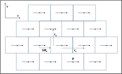
Figure 1. Brickstone lattice of transition dipoles, modelling a 2D J-aggregate.
Download figure:
Standard image High-resolution imageIn these simulations, of particular interest is how the couplings and hence exciton dynamics changes as a function of the distance between the molecular centres. A series of different separation vectors,  and
and  are used, namely, rx = ry = 2 nm, rx = ry = 5 nm and rx = ry = 10 nm. The resulting 2D lattice for the first case has approximate dimensions of 50 nm by 50 nm, with 25 molecules in each direction. The other grids are scaled proportionately. The electronic excitation energy for the molecules in this work was taken to be 3 eV and therefore the reduced wavelength is approximately 66 nm.
The electronic coupling terms were then calculated for every pairwise interaction by employing equations (10) and (13) for the QED and Förster terms respectively. The transition dipole moments of the molecules were taken to be 10.0 D, which is consistent with the types of molecules that make thin film aggregates [40]. All dipoles are centred at the lattice points and oriented along the x-direction and hence parallel to one another.
In the case of the Förster coupling, the orientation factors between each of the pairs are calculated using equation (14). The coupling itself, VF, is then calculated using equation (13). The QED coupling, VQED, is calculated by contracting the electromagnetic coupling tensor, equation (12) with the transition dipole moments of the donor and acceptors, equation (10). The density matrix is initialized with the full population localised on the central molecule of the lattice.
3. Results
The focal point of this work is the investigation of both spatial and temporal deviations between exciton dynamics driven by electronic couplings calculated from Förster theory and those calculated from the unified theory of EET. Of particular interest in this work is the importance of the intermediate-and far-zone terms that appear in the electromagnetic coupling tensor and how this is reflected through equation (10). This theoretical investigation is motivated by several studies that have noted deviations from Förster theory's characteristic  dependence on the rate of EET (the rate of EET is proportional to the square of the coupling) [41–43]. Any deviations from Förster theory could have an impact on design strategies for the development of mesoscopic energy harvesting materials [47–59].
3.1. The electronic coupling landscapes
For the case of the brickstone lattice, the electronic coupling landscapes derived from both Förster theory and QED, between the central molecule of the lattice and each of the other molecules is shown in figure 2. Each of the terms for the QED derived couplings, that is the  ,
,  and
and  dependent terms are considered independently. The total couplings for the Förster and QED cases are also considered.

Figure 2. Coupling magnitudes (on logarithmic scale) between the central molecule and all other molecules in the aggregate for rx = ry = 2 nm. (a) Contributions to the coupling from the far-zone,  , term, (b) the intermediate-zone,
  term, (c) the near-zone,
  , (d) the Förster coupling, (e) the full QED coupling and (f) the difference in (logarithms of) the QED and Förster couplings. Note that figure (f) has a different scale to the others.
Download figure:
Standard image High-resolution imageFrom the bottom part of figure 2 it is evident that the couplings derived from Förster theory and QED are very similar. In both cases there are regions of very strong coupling at short ranges. Keeping in mind that the transition dipoles are aligned parallel to the x-axis, the shape of the red region implies that molecules are coupled by mediating photons with fields that have both transverse and longitudinal character. Fields of longitudinal character most strongly couple transition dipole moments that are parallel to one another and also parallel to the displacement vector. Fields of transverse character couple transition dipole moments that are parallel to one another, but perpendicular to the displacement vector. Although not easily obvious to the naked eye when considering the bottom plots in figure 2, it is clear from the top panels that the  and
and  terms contribute to the QED coupling. As the
  and
and  terms have a common orientation factor,
  , the shape of their coupling landscapes, figures 2(b) and (c) are identical, but with the intermediate-zone
  more strongly damped at short distances. In the case of the far-zone
  coupling, there is no coupling between the central molecule and other molecules at y = 0 nm, this is because there is no contribution from longitudinal fields in the far-zone coupling term. The far-zone coupling is dominated by photons with transverse fields, and hence the coupling fans out along the y-coordinate. It is also interesting to note the St Andrew's cross like region of very low coupling for the
  and
and  landscapes. This exists because molecules coupled in this orientation are not strongly coupled by either transverse or longitudinal fields. For deeper accounts of photon coupling, the reader is pointed elsewhere [46].
3.2. Quantum dynamics—closely packed lattice; Rx = Ry = 2 nm
In this section, the coupling terms associated with the Förster and QED theories are investigated by considering exciton dynamics on a 25 × 25 brickstone lattice. The lattice has dimensions of approximately 49 nm × 48 nm. The electronic excitation energy associated with each site and therefore the energy of the transferring UV photon is taken to be 3 eV. The electronic energy transfer processes is initialized such that a site close to the centre of the brickstone lattice initially has 100% exciton density.
Figures 3 and 4 display the results of the quantum dynamics simulations. Figure 3 corresponds to simulations that employ electronic couplings derived from Förster theory, and figure 4 corresponds to simulations based on QED derived couplings. The figures are contour plots of the population of the exciton density over the lattice, at selected times during 100 fs trajectories. Figure 5 shows the exciton population data at selected sites in the lattice as a function of time for the VQED simulations.

Figure 3. Logarithmic plots of the exciton population at selected times during the dynamics simulation using the Förster theory coupling VF.
Download figure:
Standard image High-resolution image
Figure 4. Logarithmic plots of the exciton population at selected times during the dynamics simulation using the QED theory coupling VQED.
Download figure:
Standard image High-resolution image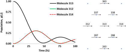
Figure 5. Populations at central sites as a function of time using the QED theory, with rx = ry = 2 nm. Central site + the site either side numbering about central site (right).
Download figure:
Standard image High-resolution imageFrom figures 3 and 4 it can be seen the dynamics derived from Förster theory agree well with the accurate QED description, for lattices of this type, where the TDM's are 2 nm apart. The migration of the exciton energy is anisotropic, as already predicted in reference [37] for these kinds of lattice geometries. The population spreads out from the centre of the lattice in both the x and y directions, with the predominant axis of exciton transport being that of the x-axis. These favoured directions of energy transfer can be explained through the coupling depictions described previously, where there is significant longitudinal character of the fields associated with the photons and hence the exciton moves more rapidly along the x-direction than the y-direction. Early on in the trajectory (at 2 and 20 fs) the spatial dependence of the population at the sites in the lattice matches well between both theories. This can be clearly seen in the similarities of the shapes of the coupling diagrams described by the Förster and QED theories. As the dynamics continues, the regions of low population that were present along the diagonal directions from the centre of the lattice now begin to gain some exciton population. At times greater than 40 fs the spatial dependence now takes on more of an elliptical shape as the population of exciton energy increases further out into the lattice. From figure 5 the symmetrical nature of the transfer of energy can clearly be seen. Figure 5 (left) shows how the population at the central site decays, before gaining exciton population after around 50 fs, and then falling away once more, characteristic of the wavelike motion of the exciton diffusion process. It can also be seen that the increase in exciton population of the nearest neighbours to the central site lying in the positive and negative x-direction (sites 312 and 314) are strongly correlated to the decay of population at site 313. This is consistent with the illustrations from the contour plots that energy is transferred in the direction of maximum coupling.
From the quantum dynamical results it can be seen that there does not appear to be any significant difference in either the spatial or temporal dependence of the exciton dynamics using electronic couplings derived from the two different theories. To corroborate this, figure 6 displays the difference between the contour plots given in figures 3 and 4.

Figure 6. Plots of the difference in the logarithm of the exciton population between the two theories at selected times during the dynamics. A value of 0 indicates that there is no difference between the populations resulting from the two theories and is shown in the plots by a sky blue colour. The positive values indicate that the QED theory results in a greater population, while a value less than 0 signifies that the Förster theory results in a greater population.
Download figure:
Standard image High-resolution imageA value of 0 in the plots of figure 6 is represented by a sky blue colour which indicates that there is no significant difference in the populations at those sites in the lattice. A value greater than 0 implies that the QED theory gives rise to a larger population, while a value below 0 indicates that the Förster theory produces a larger population (for a specific grid point and time). Looking at all panels of figure 6, the population change that occurs in the central region of the lattice is the same for the two models of energy transfer, Förster and QED. This quantitatively shows that the two theories are consistent with one another in the near-zone, at least for the lattice parameters employed here. However, small differences in the spatial dependency of energy transfer for Förster and QED derived couplings can be clearly seen in some regions of the lattice at early times. The difference then becomes 'washed-out' as time goes on, and the exciton populations eventually reach equivalence. This occurs because far-zone coupling (the R−1 distant dependent term in equations (10) and (12)) dominates at early times when direct transfer of population occurs between the initially populated central site and molecular centres at the periphery of the lattice. It is important to keep in mind that the spatial dependence of the far-zone coupling term is significantly different to the other terms because it is coupled solely by transverse photons. The far-zone coupling spreads out in the y direction because transition dipole moments that are perpendicular to each other and also perpendicular to the displacement vector are coupled.
Although one may naively expect the exciton dynamics produced by QED theory to result in a faster population transfer and hence greater population at greater distances, Förster theory in fact yields a larger population before the 40 fs point of the trajectory in some regions of the lattice (the dark blue regions of the figures). Contributions from the intermediate-zone interactions explain why the Förster coupling shows larger populations at some sites in the lattice during the trajectory. Consideration of the retarded dipole–dipole electromagnetic coupling tensor, equation (12), reveals that the R−2 contribution is taken away from the R−3 term. Consequently a weaker coupling results between the central molecule and those molecules that are most strongly coupled by the intermediate-zone coupling term. Hence a greater population is seen at early times when the Förster coupling is employed. At times > 40 fs, these differences begin to disappear and the two theories become increasingly consistent with one another. Interestingly, this is about the same time scale that corresponds to the change in shape of the contour plots in figures 3 and 4, where the distinct low population diagonal regions are lost and a more elliptical shape is formed. This can be interpreted as the exciton dynamics becoming dominated by the short range 'hopping' mechanism induced by the near-zone coupling. In effect, the short range mechanism eventually catches up to the longer range contributions to the dynamics and begins to wash-out the effects of the R−2 and R−1 terms in the QED coupling. As explained before, the R−2 term dominates when  and this occurs when the donor-acceptor separation distance, R, is approximately equal to the reduced wavelength of the mediating virtual photon. The electronic excitation energy for the molecules in this work was taken to be 3 eV and therefore the reduced wavelength is approximately 66 nm. For these simulations in which lattice parameters of 2 nm have been employed with a 25 × 25 grid, the distance over which exciton diffusion is able to occur does not exceed the reduced wavelength of the mediating virtual photon, except at the outskirts of the diagonal regions of the lattice. Thus, although the intermediate and far-zone terms have a clear effect, neither term has a lasting influence on the dynamics of energy transfer. Consequently the quantum dynamics derived from couplings calculated with Förster theory are largely consistent with those derived from coupling calculated from QED.
3.3. Quantum dynamics—sparsely packed lattices; Rx = Ry = 5 nm and Rx = Ry = 10 nm
The first of these scenarios employs the same brickstone lattice model and transition dipoles used above, but with 5 nm between the rows and 5 nm between the monomers in the x direction. By employing the 25 × 25 grid as before, the dimensions of the lattice become approximately 122 nm × 120 nm. Figures 7 and 8 show contour plots of the exciton population at selected times during the simulations using the Förster and QED theories respectively (logarithmic scale).
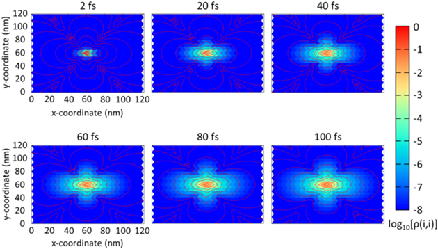
Figure 7. Logarithmic plots of the exciton population at selected times during the dynamics simulation using the Förster theory for lattice parameters Rx = Ry = 5 nm.
Download figure:
Standard image High-resolution image
Figure 8. Logarithmic plots of the exciton population at selected times during the dynamics simulation using the QED theory for lattice parameters Rx = Ry = 5 nm.
Download figure:
Standard image High-resolution imageThe first thing to note from these results is that the rate at which energy migrates from the central site is much slower than in the case of the 2 nm spaced lattice. Figures 7 and 8 both show similar qualitative features, as those shown in figures 3 and 4. That is, the exciton migration is anisotropic, with the principal axes of transfer occurring along the directions of maximum coupling. However, due to the increased lattice size, the elliptical shape seen after around 40 fs in the case of the 2 nm spaced lattice is not seen here. Instead the distinctive spatial dependence remains throughout the dynamics. This is a consequence of the fact that there is a much slower rate of energy transfer and hence the population actually transferred is small on the time scale of these simulations. The final population recorded at the central site for both theories is approximately 0.95 at 100 fs.
The exciton dynamics plots, figures 7 and 8, once again seem to suggest that the results from QED coupling qualitatively match the result from the Förster coupling. However there are clear differences when one looks at the population difference plot (figure 9), suggesting that the intermediate- and far-zone terms are starting to have a sustained influence on the exciton dynamics when the distance between the centres is approximately greater than 5 nm.

Figure 9. Plots of the difference in the logarithm of the exciton population between the two theories at selected times during the dynamics for the 5 nm lattice.
Download figure:
Standard image High-resolution imageFigure 9 shows similar topographies as those for the 2 fs time in figure 6, although the features are now significantly more prominent and long lasting, with differences persisting to the 100 fs mark. It can be clearly seen that the narrow regions protruding diagonally out from the initially excited molecule favour exciton transport described by QED coupling, while the triangular regions above and below the central point predict slower exciton transport for QED coupling than Förster coupling. This contrast between the exciton dynamics resulting from QED derived couplings and those of Förster theory becomes even larger when the separation between the dipole centres increases (to 10 nm), as can be seen in figures 10–12.

Figure 10. Logarithmic plots of the exciton population at selected times during the dynamics simulation using the Förster theory for lattice parameters Rx = Ry = 10 nm.
Download figure:
Standard image High-resolution image
Figure 11. Logarithmic plots of the exciton population at selected times during the dynamics simulation using the QED theory for lattice parameters Rx = Ry = 10 nm.
Download figure:
Standard image High-resolution image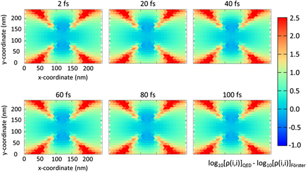
Figure 12. Plots of the difference in the logarithm of the exciton population between the two theories at selected times during the dynamics for the 10 nm lattice.
Download figure:
Standard image High-resolution image
Looking at the outer regions of the lattice in the plots in figures 9 and 12, one can see that there are more significant differences between the two coupling theories in describing the population dynamics as the distance between the sites spread out. Importantly, the results also show that the differences are no longer washed out as quickly as they were with the lattice with 2 nm spacings between molecules. This indicates that intermediate and far-zone terms for the QED coupling are starting to play an important role in the dynamics of energy transfer for molecules separated by these distances. In terms of the spatial dependence, it can be seen that regions of differences form a very distinctive pattern. The fact that the areas of these plots in which the QED coupling is shown to result in a larger population occur along the diagonal regions emanating from the centre of the lattice, indicate that it is the R−1 term that is contributing at these sites. As explained before, the origin of these diagonal features is in the fact that the far-zone coupling term seen in equation (12) has a different orientational dependence. Again there are regions in which the Förster coupling yields larger populations, originating from the intermediate-zone, R−2 term, which is subtracted from the R−3 near-zone term in these regions of the lattice. In a similar trend to the results of the lattice with molecules separated by 2 nm, some of the population differences are washed out with time. For example on the outskirts of the diagonal regions of the lattice where the Förster theory dynamics approaches the same population as the QED coupling dynamics at later times. However convergence of exciton populations of the two theories does not occur. For example, there are parts of the lattice, above and below the central region (where the intermediate-zone term dominates) in which the Förster theory appears to produce a greater population as time goes on (i.e. it becomes less realistic in these regions). This is presumably because the influence of the intermediate-zone R−2 term dominates over these specific distances and orientations. It is especially interesting to note that even though these distances are significantly shorter than the reduced wavelength of the mediating photon (approximately 66 nm for these simulations), the R−2 contribution to the QED coupling plays a significant role at early times, within the context of these simulations.
In closing this section, it is important to point out that while the absolute differences in the populations may in fact be quite small in magnitude, this is largely because the EET dynamics is undertaken on lattices of 625 molecules. Consequently the absolute population that any of the molecular centres possesses, especially near the periphery of the grids, where the deviations between Förster theory and the unified theory of EET are most apparent, will be very small. Nevertheless, as can be seen clearly from the figures, the exciton dynamics is significantly different. The differences will be compounded when the number of molecular centres is reduced and it is expected that these differences will be especially important for energy transfer between two species, as is the case in many FRET studies.
4. Conclusions
In this work, the electronic coupling terms associated with the Förster theory of energy transfer and the unified theory of EET have been investigated. The analysis considered the spatial dependence of the coupling terms themselves as well as through a quantum dynamical approach for simulating the process of electronic energy transfer in a brickstone lattice. The coupling term associated with the Förster theory, equation (13), and the transition matrix element associated with the unified theory, equation (10), are employed as off-diagonal coupling terms in the site basis Hamiltonian. The Liouville–von Neumann equations of motion were used to propagate the exciton density matrix. The focus throughout this investigation was to study the difference between the ensuing exciton dynamics, based on the two different coupling methods. Of particular interest is the role that intermediate- and far-zone terms play in the spatial and temporal dynamics.
The results revealed that for closely spaced lattices, in which the distances between the points of an array are 2 nm, the QED theory is consistent with the Förster theory. It was found that by increasing the size of the lattice simply by increasing the distance between the transition dipole moments in the array, the intermediate- and far-zone contributions to the couplings start to play important roles in the spatial and temporal exciton dynamics. In some regions of the lattice greater populations were seen when QED couplings were employed, and in other regions smaller populations resulted at specific times.
The differences in the resulting dynamics became more pronounced as the distance between the transition dipole moments became greater. In the case where rx and ry = 2 nm, any deviations between the dynamics driven by VF and VQED were quickly washed-out. As the distance between the molecular centres increased, the exciton dynamics driven by QED couplings diverged significantly from the dynamics of Förster theory for the full 100 fs.
These results indicate that intermediate-zone and even far-zone terms may be important in accurately describing exciton movement in mesoscopic structures, where EET can occur over tens of nanometres, such as quantum-dot arrays. However more ab initio quantum simulations will be required to verify how significant this is for realistic structures. Further, there may be implications for the application of spectroscopic ruler techniques, with a number of experimental studies recently predicting deviations from the usual R−6 dependence on the rate of EET [41–43, 59].
Acknowledgements
The work was in part funded by the Engineering and Physical Sciences Research Council (UK) (EPSRC(GB)) (G.A.J., EP/K003100). We thank Professor David Andrews for continuing stimulating discussions and proof reading the manuscript. The research presented in this paper was carried out on the High Performance Computing Cluster supported by the Research and Specialist Computing Support service at the University of East Anglia.
Footnotes
- 2
The reason for this is that there are two possible Feynman diagrams associated with the energy transfer process. However, only one results in the conceptually attractive view of the virtual photon being created as the donor falls into its ground state.