


Abstract
Differential interferometry (DI) with two coupled sensors is a most powerful approach for precision measurements in the presence of strong phase noise. However, DI has been studied and implemented only with classical resources. Here we generalize the theory of differential interferometry to the case of entangled probe states. We demonstrate that, for perfectly correlated interferometers and in the presence of arbitrary large phase noise, sub-shot noise sensitivities—up to the Heisenberg limit—are still possible with a special class of entangled states in the ideal lossless scenario. These states belong to a decoherence free subspace where entanglement is passively protected. Our work paves the way to the full exploitation of entanglement in precision measurements.
Export citation and abstract BibTeX RIS

Content from this work may be used under the terms of the Creative Commons Attribution 3.0 licence. Any further distribution of this work must maintain attribution to the author(s) and the title of the work, journal citation and DOI.
1. Introduction
Atom interferometers [1] nowadays offer unprecedented precision in the measurement of gravity [2], inertial forces [3], atomic properties [4], and fundamental constants [5]. Their large sensitivity makes their coupling to the environment almost unavoidable, which mainly results in a random noise which affects the signal phase. In order to overcome this limitation, many experiments aiming at precision measurements adopt a differential scheme: two interferometers operating in parallel are affected by the same phase noise and accumulate a different phase shift induced by the measured field. Estimation of the differential phase allows high resolution, thanks to noise cancellation [6]. Schemes based on this concept have proven crucial for the precision measurement of rotations [7], gradients [8], and fundamental constants [9]. Differential atom interferometers have also been proposed for tests of general relativity [10], equivalence principle [11], atom neutrality [12], and for detection of gravitational waves [13]. So far, differential interferometry (DI) has only been exploited with classical resources. Its sensitivity is thus ultimately bounded by the shot noise (SN) limit,  , where N is the number of particles in the input. For the single interferometer operation, a significant enhancement of phase sensitivity up to the Heisenberg limit (HL)
  can be obtained by using particle-entangled input states [14–17]. This prediction is under intense experimental investigation with cold [18] and ultracold [19–24] atoms. However, the analysis of a single interferometer has emphasized [25–29] that sub-SN cannot be reached in presence of strong phase noise. Is it possible to exploit DI with highly entangled states to overcome the SN5
in such a noisy environment?
can be obtained by using particle-entangled input states [14–17]. This prediction is under intense experimental investigation with cold [18] and ultracold [19–24] atoms. However, the analysis of a single interferometer has emphasized [25–29] that sub-SN cannot be reached in presence of strong phase noise. Is it possible to exploit DI with highly entangled states to overcome the SN5
in such a noisy environment?
In this manuscript we study DI with two sensors implementing quantum resources and affected by phase noise of an arbitrarily large amplitude (see figure 1)6 . Our analysis takes into account the correlations of the two interferometer outcomes. It goes beyond the trivial subtraction of the two output phases estimated independently, which does not offer any significant quantum enhancement of phase sensitivity. We provide the necessary and sufficient condition, based on the Fisher information, for an entangled state to allow sub-SN phase sensitivity. We also demonstrate that the HL, which is believed to be achievable only in noiseless quantum interferometers [25–28], is preserved by the lossless differential scheme, as long as relative noise fluctuations are also at the HL. While the HL is saturated by maximally entangled states that are extremely fragile to particle losses, the SN can be overcome by less entangled and more robust states, such as those experimentally created via particle–particle interaction in Bose–Einstein condensates (BECs) [19–24]. These findings open the door to full exploitation of quantum resources in realistic devices, provided that a DI scheme is implemented.
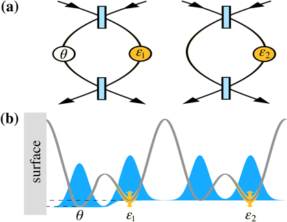
Figure 1. Differential scheme discussed in this manuscript. (a) Two Mach–Zehnder interferometers affected by shot-to-shot random phase noise  and
and  . The signal θ can be estimated in the presence of arbitrary noise, provided that relative noise fluctuations are sufficiently small. (b) Application to Bose–Einstein condensates (with spatial density represented by blue filled regions) trapped in a superlattice potential (gray curve). Splitting operations in each double-well are obtained by tuning the inter-well barrier. Short range forces between atoms and a nearby surface induce a phase shift
  . Trapping-potential fluctuations lead to correlations between
  and
and  .
.
Download figure:
Standard image High-resolution image2. Parameter estimation in differential interferometry
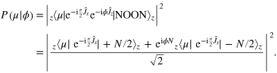
Figure 1(a) shows the general DI scheme discussed in this manuscript. It consists of two interferometers running in parallel. The input state  is transformed by
  , where
  are collective spin operators for the first and second interferometer, respectively. The phase shift in the first (second) interferometer is
  (
( ), where θ is the 'signal phase' to be estimated and
 ![${{\epsilon }_{1}},{{\epsilon }_{2}}\in [-\pi ,\pi ]$](https://content.cld.iop.org/journals/1367-2630/16/11/113074/revision1/njp503338ieqn13.gif) is the phase noise accumulated during the interferometer operations. The values of
is the phase noise accumulated during the interferometer operations. The values of  and
and  change randomly in repeated shots, with probability distribution
  . Our general formalism does not assume a specific noise model and encompasses both Markovian and non-Markovian dephasing [we will later discuss specific forms of
  and focus on the case of a correlated interferometer, where
  ]. We consider a general positive-operator value measure (POVM)
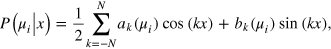
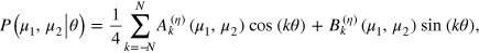
  on the output state and use an unbiased estimator
  , which is a function of the results obtained in m repeated independent measurements [36]. The variance of the estimator fulfills
  [34], where

is the the Cramer–Rao (CR) bound,
is the Fisher information (FI),

are conditional probabilities, and ![$P(\mu |\theta ,{{\epsilon }_{1}},{{\epsilon }_{2}})={\rm Tr}[\hat{E}(\mu )\hat{U}(\theta ,{{\epsilon }_{1}},{{\epsilon }_{2}})\hat{\rho }{{\hat{U}}^{\dagger }}(\theta ,{{\epsilon }_{1}},{{\epsilon }_{2}})]$](https://content.cld.iop.org/journals/1367-2630/16/11/113074/revision1/njp503338ieqn22.gif) . In particular, if the state
. In particular, if the state  is separable in the two interferometers,
  , and the measurements in each interferometer are independent,
  [
[ ], then equation (3) becomes

Equation (1) takes into account the full quantum correlations of the interferometers outcomes and provides the lowest possible phase uncertainty, given the conditional probability distribution  . It can be saturated for large m by the maximum-likelihood estimator [34].
3. Phase sensitivity
Here we calculate the highest sensitivity allowed by the above DI scheme. We rewrite equation (3) as ![$P(\mu |\theta )={\rm Tr}[\hat{E}(\mu )\hat{U}(\theta ){{\hat{\rho }}_{{\rm eff}}}{{\hat{U}}^{\dagger }}(\theta )]$](https://content.cld.iop.org/journals/1367-2630/16/11/113074/revision1/njp503338ieqn28.gif) , where
, where  depends solely on θ and

The noisy differential interferometer with input  is thus equivalent to a noiseless interferometer with effective input density matrix
  . This equivalence can be used to minimize
  over all possible POVMs [35, 36]. We have
where ![${{F}_{Q}}[{{\hat{\rho }}_{{\rm eff}}}]=4{{(\Delta \hat{R})}^{2}}$](https://content.cld.iop.org/journals/1367-2630/16/11/113074/revision1/njp503338ieqn33.gif) is the quantum Fisher information (QFI) and
is the quantum Fisher information (QFI) and  is obtained by solving
 ![$\{\hat{R},{{\hat{\rho }}_{{\rm eff}}}\}=i[{{\hat{\rho }}_{{\rm eff}}},{{\hat{J}}_{1}}\otimes {{1}_{2}}]$](https://content.cld.iop.org/journals/1367-2630/16/11/113074/revision1/njp503338ieqn35.gif) . Taking
. Taking  the eigenbasis of
  [
[ ,
,  ], where
  labels the interferometer, we have

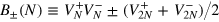
where

Depending on  , the DI may admit a decoherence free subspace (DFS) spanned by states of the system that experience no evolution under the noise7
. For uncorrelated noise [
, the DI may admit a decoherence free subspace (DFS) spanned by states of the system that experience no evolution under the noise7
. For uncorrelated noise [ ], we obtain
  if and only if
  ; i.e., the DFS simply reduces to the eigenstates of
  . These states are insensitive to the phase shift and thus useless for phase estimation. As common in several differential atom interferometers, we assume that
  , where
  indicates the total ('+' sign) and relative ('-' sign) noise. Equation (8) becomes

where  . A non-trivial DFS, defined by the condition
  [
[ ], exists in the limit of vanishing relative
  [total,
  ] noise fluctuations. Such a DFS can be decomposed in subspaces defined by constant values of
  [
[ ]. These, except the trivial case
  , contain coherence terms and are thus relevant for phase estimation. For vanishing total (relative) noise and in presence of large relative (total) noise,
  becomes block diagonal (see figure 2(a)), describing a statistical mixture of states with definite M values. We thus write
  , where
  ,
,  are projectors into the fixed-M subspace, and
 ![${{Q}_{M}}={\rm Tr}[{{\hat{\pi }}_{M}}\hat{\rho }{{\hat{\pi }}_{M}}]$](https://content.cld.iop.org/journals/1367-2630/16/11/113074/revision1/njp503338ieqn60.gif) are weights satisfying
are weights satisfying  . We have
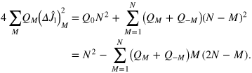
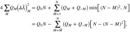
 ![${{F}_{Q}}[{{\hat{\rho }}_{{\rm eff}}}]\leqslant {{\sum }_{M}}{{Q}_{M}}{{F}_{Q}}[{{\hat{\rho }}_{M}}]\leqslant 4{{\sum }_{M}}{{Q}_{M}}(\Delta {{\hat{J}}_{1}})_{M}^{2}$](https://content.cld.iop.org/journals/1367-2630/16/11/113074/revision1/njp503338ieqn62.gif) , where
, where  is the variance of
  calculated for
  , and the second bound can be saturated by pure states. For separable states, following [16] and assuming, for simplicity,
  , we have

where  is the solution of
  . In general,

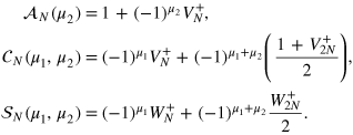
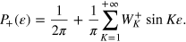
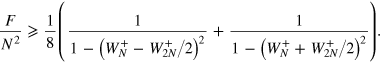
In equations (10) and (11), the QFI is maximized by populating only the M = 0 subspace. We recover the same phase uncertainty bounds as in the ideal noiseless case: the SN limit,  , for separable states, and the HL,
  , for general quantum states. In other words, the condition
 ![${{F}_{Q}}[{{\hat{\rho }}_{{\rm eff}}}]\gt N$](https://content.cld.iop.org/journals/1367-2630/16/11/113074/revision1/njp503338ieqn71.gif) is necessary and sufficient for reaching sub-SN sensitivities. Moreover, according to equation (10), overcoming the SN necessarily requires particle entanglement in the effective input state. In full analogy to the noiseless case, there exist optimal entangled states providing a quadratic enhancement of phase sensitivity even in the presence of large phase noise. The optimal states for DI are (in the
is necessary and sufficient for reaching sub-SN sensitivities. Moreover, according to equation (10), overcoming the SN necessarily requires particle entanglement in the effective input state. In full analogy to the noiseless case, there exist optimal entangled states providing a quadratic enhancement of phase sensitivity even in the presence of large phase noise. The optimal states for DI are (in the  basis, see figure 2(b))
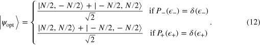
These have  and are not affected by phase noise. The states (12) have been experimentally realized with two [39] and up to eight [40] trapped ions and further investigated in [41]. While the saturation of the HL requires entangled interferometers, we can still have an HL scaling, i.e.,
  , if we consider states which are separable in the two interferometers
  . A prominent example is the product of NOON states,

which, as shown in figure 2(c) does not (entirely) belong to the DFS and has  both when
  and when
  .
.
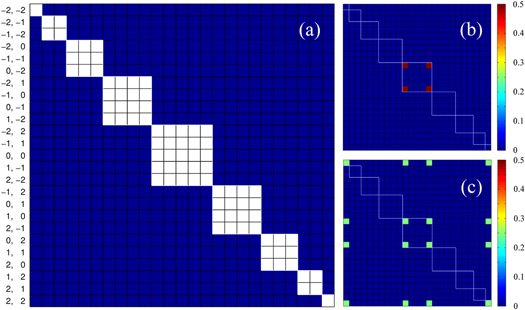
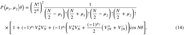
Figure 2. Panel (a) shows the general layout of a density matrix  of four particles in each interferometer. The basis indexes n1, n2 are reported on the left part of the figure. Following an opportune reordering of the basis, the DFS for vanishing relative noise fluctuations
  is shown by the white squares corresponding (from top-left to bottom-right) to
  . Panel (b) shows the density matrix of state (12), fully included in the central (M = 0) DFS. Panel (c) shows the density matrix of state (13). In the left panels the color scale is
  .
.
Download figure:
Standard image High-resolution image4. Differential interferometry with NOON states
In this section we study the DI scheme  , each interferometer being represented by a phase shift rotation around the z axis followed by a 50–50 beam splitter. We further assume the phase noise distribution
 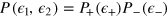 . As an input state we take the direct product of NOON states,
  , with components along the z direction,
  [42],
[42],  being an eigenstate of
  with eigenvalue
  . In the following we provide the conditional probabilities and FI when
  are even functions of
  and specialize to the case a Gaussian noise distribution. For a discussion on more general noise functions, see appendix
The probability of measuring a relative number of particles  at the output of interferometer 1 and
  at the output of interferometer 2 can be calculated analytically and is given by (see appendix
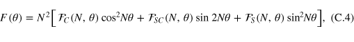
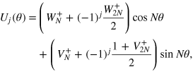
where 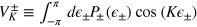 . The FI is
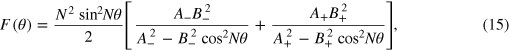
where 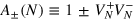 ,
,  . The optimal value of the FI,
  , is reached for
  ,
,
Let us discuss the different limit values of equation (16), taking into account that  when
when  and
and  when
when  . If relative noise fluctuations are vanishingly small,
  , equation (16) ranges from
  (if also
  , corresponding to the ideal noiseless limit) to
  (when
(when  ). In other words, if the relative noise between the two interferometers is fixed, a phase sensitivity at the HL can be obtained for an arbitrary large total noise (i.e., arbitrary large noise in each interferometer). If total noise fluctuations are large,
  , we obtain
  , which predicts the HL for
  and sub-SN for
  . In figure 3(c) we plot equation (16) as a function of
  , taking
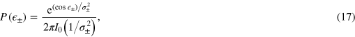
where  is the modified Bessel function of the first kind. This noise function continuously interpolates from a Gaussian distribution of width
  , when
  , to a flat distribution, when
  . The condition
  is thus equivalent to
  , while
  is recovered for
  . These results show that reaching the HL in the differential interferometer requires relative noise fluctuations at the HL itself.
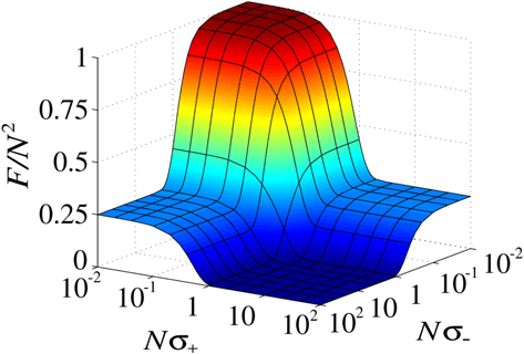
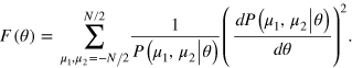
Figure 3. FI (maximized over  ) for a differential interferometer with noise distribution given by equation (17) and factorized NOON states in equation (13) as input (see text for details). Here N = 100.
Download figure:
Standard image High-resolution image5. Precision limit for differential interferometery with Bose–Einstein condensates
In this section we discuss a differential Mach–Zehnder (MZ) interferometer  with input states that can be created with two-mode BECs. We consider phase estimation from the measurement of the number of particles in output. We further take vanishing relative phase noise fluctuations in the two interferometers,
  , and
, and  , given by equation (17).
We first consider adiabatic state preparation [43], focusing on the ground state  of the Hamiltonian
  , with
  . This can be implemented in a double-well trap (see figure 1(b)) with
  and Ω interaction and tunneling parameters, respectively [19, 22]. We can distinguish Rabi
  , Josephson
  , and Fock
  regimes. In the ideal case, these regimes are characterized by different scalings of the FI (optimized in
  ):
):  (F = N for the spin coherent state,
  ,
,  ),
),  , and
, and  ∼ N2 (
 [44] for the twin-Fock state,
  ,
,  ), respectively [45]. In figure 4(a) we report the FI (optimized in θ) as a function of Λ for the differential MZ with input
  . Different lines refer to different values of
  , ranging from the noiseless case (
 , thick dashed line) to the uniform phase noise (
 , thick solid line). The twin-Fock is optimal for
  , while for
  , the FI is maximized at
  .
.

Figure 4. (a) FI as a function of Λ for the adiabatic state preparation. The shadow regions highlight different regimes (see text). (b) FI as a function of τ for the diabatic state preparation. In panels (a) and (b), N = 100, and different lines refer to different values of  . (c) FI as a function of N for various input states of the differential MZ interferometer and
  . Solid thin lines are fits, while solid thick lines are the HL and SN (the white region between the two lines corresponds to sub-SN). (d) FI for the twin-Fock state as a function of N and for different
  values. Thick lines and colored regions are as in panel (c).
Download figure:
Standard image High-resolution imageWe further consider states that are created by the nonlinear evolution  , starting from a spin coherent state [14, 20, 46], where
  . Here
  rotates the state so to maximize the FI in the noiseless case [16]8
. In figure 4(b) we show the FI for the differential MZ with input
rotates the state so to maximize the FI in the noiseless case [16]8
. In figure 4(b) we show the FI for the differential MZ with input  . Lines are as in figure 4(a). Interestingly, the short time dynamics (
 , where spin squeezing is created [46]) is robust, and sub-SN is found also for large phase noise. The characteristic plateau (
 for the ideal case [16]) is washed out when
  . The FI at large values of
  is characterized by several peaks, the most prominent found in correspondence to the creation of macroscopic superposition states ('phase cats') with multiple (larger than two) components. The long-time dynamics at
  leads to maximally entangled states (a two-components phase cat) having
  , as discussed in the previous section.
We have repeated the previous analysis for specific input states and large values of N (up to  ) and
) and  (flat total noise case). The results are shown in figure 4(c). The FI reaches an asymptotic power law scaling
  :
:  ,
,  for coherent spin state (green diamonds);
  ,
,  for the optimal states of the adiabatic preparation at
  (red squares);
  ,
,  for the optimal states of the diabatic preparation at time
  (blue circles);
  for the twin-Fock state (black dots). The solid black line is the analytical NOON state result (
 ,
,  ) discussed previously. The twin-Fock state is an interesting and experimentally relevant [21] example. It is strongly entangled and reaches an HL scaling in the single noiseless MZ; however, it performs only slightly better than the SN in the differential MZ with large noise and a large number of particles. In figure 4(d) we further investigated the FI for the twin-Fock state as a function of N for different values of
  (dots). For
  and
and  , the FI follows the ideal behavior
  (dashed line). For
  , we recover roughly the same scaling of FI (
 ) as in the large phase noise case.
6. Conclusions
In this manuscript we have extended the analysis of DI to the domain of entangled states. It is not obvious, a priori, that DI can suppress spurious phase noise when highly entangled—and thus extremely fragile against phase noise fluctuations—states are used. Our analysis reveals that when the phase noise is perfectly correlated in the two interferometers, and losses can be neglected, there exists a DFS where entanglement is passively protected. We have thus identified a class of entangled input state that can provide a sub-SN sensitivity in a differential interferometer up to the HL, even for large noise. This class is nontrivial, fully characterized by the FI, and includes states that have been recently created experimentally. We expect our results to be a guideline for quantum-enhanced realistic interferometers in the near future.
Acknowledgments
This work has been supported by the EU-STREP Project QIBEC and ERC StG No. 258325. LP and MF acknowledge financial support by MIUR through FIRB Project No. RBFR08H058.
Appendix A.: Derivation of equation (3)
We here derive equation (3) from first principles. We start from the joint probability density  and integrate over
  and
and  ,
,

so as to eliminate nuisance parameters. By using the relation  between joint and conditional probabilities, where x and y are random variables, we have

Since  do not depend on
  , i.e.,
  , we recover equation (3).
Appendix B.: Derivation of inequalities (10) and (11)
Here we detail the calculation of  , where
  is the variance of the operator
  calculated on the fixed-M subspace. We consider the case
  for simplicity. We have
  , where
 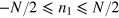 are the eigenvalues of
  and
and  (
( ) are the maximum (minimum) values of n1 in the fixed-M DFS. In general,
  , and
, and  . We thus have

where equality of  is the equal-weighted superposition of states with the maximum and the minimum value of n1 in the fixed-M DFS. Taking into account that
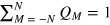
We thus recover equation (11). Since  , the second term in the equation above is nonnegative, and we find
  . For separable states, we need to further take into account that
  [16]. We thus have

and obtain
which follows, since for  we have
 ![${\rm min} [N,{{(N-M)}^{2}}]={{(N-M)}^{2}}$](https://content.cld.iop.org/journals/1367-2630/16/11/113074/revision1/njp503338ieqn205.gif) . We recover equation (10). Since for
. We recover equation (10). Since for  , we have
  . The second term in the above equation is nonnegative, and we have
  for separable states.
Appendix C.: Extension of the discussion of section 4 to arbitrary noise distributions
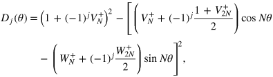
Here we provide a detailed derivation of the equations presented in section 4 and extend the discussion to arbitrary noise distributions. Let us first calculate the conditional probability distribution of the relative number of particles for the single interferometer with a NOON probe state:
The rotation matrix elements  are given by
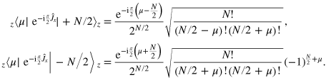
We thus obtain
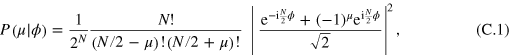
with
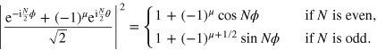
We now consider the differential sensor described by the unitary operator  , each interferometer being given by the transformation
  , i = 1,2, ϕ1 = θ +
  1 and ϕ2 = 2. We take a NOON state of N particles as the input of each interferometer (without loss of generality, we assume N to be even) and estimate the phase shift from the measurement of the relative number of particles at the output ports of each interferometer,
  . Taking
  , where
  , equation (4) writes
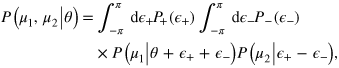
with  (i = 1,2) given by equation (C.1). After straightforward algebra, we obtain
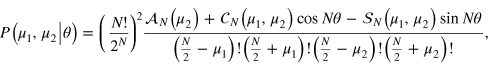
where
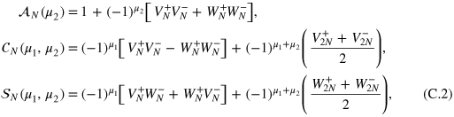
and

K being an integer number. We are now ready to compute the FI, equation (2),
The FI can be written as the sum of three terms:
where the coefficients  ,
,  , and
, and  are functions of N and
  and are given by sums over
  and
and  . To compute the sums, we separate the sum over
  into the sum over odd
  and sum over even
  (since N is assumed to be even,
  and
and  are integer numbers) and take into account that

We thus obtain
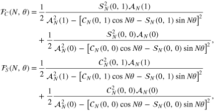
and
The above equations allow us to calculate the FI, given arbitrary relative and total noise functions. For the case of NOON input states considered here, the FI ultimately depends on the eight Fourier coefficients  ,
,  ,
,  , and
, and  . Below, we first show how the calculation of the FI simplifies when noise distributions are even functions of
  . Furthermore, we study the case of perfectly correlated relative noise and arbitrary total noise distribution.
Symmetric noise distributions. If  are even functions of
  , the calculation of the Fisher information simplifies notably. We have
  , which implies
  for all
  and
and  ,
,  , and
, and  . We also have
  ,
,  ,
,  , and
, and  , where
  and
and  have been introduced in section 4. The conditional probability and the FI reduce to equations (14) and (15), respectively.
Perfectly correlated relative noise. In the following we consider the ideal case of perfectly correlated relative noise,  . This implies
  ,
,  , and equations (C.2) simplify to
These equations are the basis for further considerations. For instance, if  (we indicate
  to simplify the notation) is an odd function of
  plus a constant providing normalization in the
  interval, then
  , and we can expand it in Fourier series as
The condition  implies
 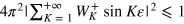 , which, integrating over
  , gives
  . In this case, evaluating
  at phase values θ such that
  , we have (we recall that
  )
)
The term between brackets does not diverge because of the condition  , and it is always larger than two. It implies that in this case,
  . To treat a more general case, we consider the noise distribution

which is a normalized sum of M peaks of width σ (for 
 , the
, the  function being used to take into account the
  -periodicity) centered at random positions
 ![${{x}_{1}},{{x}_{2}},...,{{x}_{M}}\in [-\pi ,\pi ]$](https://content.cld.iop.org/journals/1367-2630/16/11/113074/revision1/njp503338ieqn267.gif) . For random choices of
. For random choices of  , we calculate the FI and maximize over
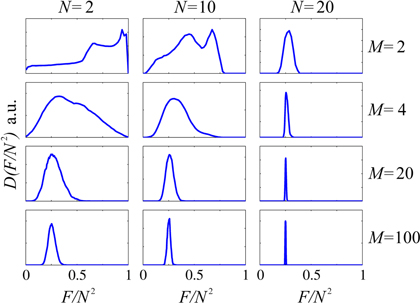
  . In figure C1
we plot the statistical distribution of
. In figure C1
we plot the statistical distribution of  as a function of N and M.
Figure C1. Statistical distribution of the  ,
,  obtained by taking equation (C.5) as (total) phase noise distribution. The different panels refer to different number of particles N (different columns) and number M of noise peaks in equation (C.5) (different rows). Here
  .
.
Download figure:
Standard image High-resolution image
For sufficiently large values of N and/or M, the noise distribution (C.5) has vanishing high frequency Fourier components. When increasing M (at a fixed value of N and  ), this is due to the fact that the noise distribution tends to become flat in most of the random realizations (i.e., for most of the random choices of
  ). When increasing N (at fixed σ and
  ), this is due to the vanishing tails in the Fourier spectrum of
  . In both cases, the coefficients
  ,
,  ,
,  , and
, and  are vanishing small, and we have

and

giving 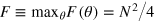 . In figure C1 we indeed observe that the distribution of F peaks around
  for sufficiently large values of N and M.
For small values of M and N, we may have a situation where  is very small. In general, for a fixed number of particles, it is possible to derive pathologic noise distributions for which the FI vanishes. To see this, it is convenient to rewrite
  as
as

with
and
with j = 0,1. Itʼs possible to demonstrate that 
 . Therefore the Fisher is zero only if both numerators are zero. It is also possible to see that the cases involving
  and
and  lead to nonphysical probability distributions. The only remaining option is to have both
 . This in turn corresponds to a probability distribution with
  ,
,  ,
,  , and
, and  . Recalling the definition of
  , we thus have that
  if and only if

This integral involves two positive functions. Equation (C.8) is thus fulfilled only if  has support in correspondence to the zeroes of
  . A total noise distribution
  for which the FI vanishes is therefore obtained, as a normalized sum of Dirac deltas symmetrically centered at the zeroes of
  . We argue that this situation is pathological for NOON states, where the FI is entirely determined by the Fourier components of
  , equation (C.3), at K = N and K = 2N. Furthermore, if
  , instead of being a sum of Dirac peaks, is a sum of peaks of finite width, we recover, as noticed above, equation (C.6) for N sufficiently large.
Appendix D.: Numerical method to compute the Fisher information
Here we report a method for the numerical calculation of the FI that we used to obtain the results of section 5. We consider a differential interferometer and indicate with  and
and  the results of a measurement at the outputs of the two devices. The differential interferometer transformation is
 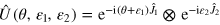 , and the joint conditional probability reads

where we have assumed  . Noticing that the functions
  , i = 1,2 are
  periodic in x, it is therefore possible to make a Fourier expansion of the functions. This is conveniently done with a fast Fourier transform algorithm. Furthermore, the discretized atom number poses a maximum allowed frequency in the decomposition given by Shannonʼs criterion:
where  and
and  are Fourier coefficients of
  . We thus find
where the coefficients are given by

and

 (and an analogous definition for
  ) are vectors of Fourier coefficients, and the matrices
  and
and  have components

respectively. Notice that it is immediate to take the derivative of equation (D.1)) with respect to θ, as required for the calculation of the FI. This is an advantage of this method.
Footnotes
- 5
Quantum-enhanced noiseless differential interferometry is studied in [30].
- 6
An optical analogous to the differential scheme discussed here (a differential Michelson-Morley interferometer with squeezed states of light as input, in particular) has been recently investigated [31]. See also quenching in a correlated emission laser, originally proposed in [32] and experimentally demonstrated in [33].
- 7
- 8
For the effect of phase noise in the state preparation see [47].