


Abstract
The electron band around the M point in the  compound, which is completely lifted up above the Fermi level for
  and hence its Fermi surface (FS) disappears, can still play the role of the main pairing resource by exchanging inter-band repulsive interaction with the main hole band (h1) around the
  point. This hidden electron band, which develops the superconducting order parameter (OP)
  but has no FS, displays a shadow gap feature which is easily detected by various experimental probes such as angle-resolved photoemission spectroscopy (ARPES) and tunneling measurements. We also show that the formation of the nodal gap
  with
with  symmetry on another hole pocket (h2) around the
  point with a larger FS is stabilized due to the balance of the inter-band repulsive interactions from the main hole band (h1) with the OP
  , and the hidden electron band with the OP
  .
.
Export citation and abstract BibTeX RIS

Content from this work may be used under the terms of the Creative Commons Attribution 3.0 licence. Any further distribution of this work must maintain attribution to the author(s) and the title of the work, journal citation and DOI.
1. Introduction
The superconducting (SC) transition is the most well known example of Fermi surface (FS) instability along with other density wave instabilities such as spin density wave (SDW), charge density wave (CDW), etc. Mathematically, it is summarized by a pairing susceptibility ![$\chi (T)=\lambda \ln [{{\Lambda }_{hi}}/T]$](https://content.cld.iop.org/journals/1367-2630/16/2/023029/revision1/njp488374ieqn12.gif) of a conduction band of the Bloch states [1], where
of a conduction band of the Bloch states [1], where  is a dimensionless coupling constant and
  is the high energy cut-off of the pairing interaction (for example,
  , Debye frequency, for phonon interaction). For the conduction band with a FS, the low energy cut-off is zero because the presence of FS allows zero energy excitations, which is replaced by T at finite temperature in the above formula. This susceptibility displays a logarithmic divergence with lowering temperature, hence no matter how weak the pairing interaction
  is, the instability condition,
  , is achieved by decreasing the temperature
 ![$T\to {{T}_{c}}={{\Lambda }_{hi}}\exp [-1/\lambda ]$](https://content.cld.iop.org/journals/1367-2630/16/2/023029/revision1/njp488374ieqn18.gif) . This is called FS instability. However, if there exists a finite low energy cut-off
. This is called FS instability. However, if there exists a finite low energy cut-off  , for example, because there is no FS, then the pair susceptibility becomes
 ![$\chi \sim \lambda \ln [{{\Lambda }_{hi}}/{{\Lambda }_{low}}]$](https://content.cld.iop.org/journals/1367-2630/16/2/023029/revision1/njp488374ieqn20.gif) and the instability condition
and the instability condition  can only be satisfied when the coupling strength
  becomes sufficiently strong, i.e.
 ![$\lambda >{{\lambda }_{crit}}=\frac{1}{\ln [{{\Lambda }_{hi}}/{{\Lambda }_{low}}]}$](https://content.cld.iop.org/journals/1367-2630/16/2/023029/revision1/njp488374ieqn23.gif) . This hypothetical exercise shows that the instability can still occur with Bloch states without the FS if the coupling is strong enough. However, notice that the susceptibility
. This hypothetical exercise shows that the instability can still occur with Bloch states without the FS if the coupling is strong enough. However, notice that the susceptibility  becomes temperature independent in this case, hence this mechanism cannot derive a phase transition in a real system by decreasing temperature. Therefore, we reconfirm the common knowledge: no FS, no phase transition with Bloch states.
In this paper, however, we demonstrate that the presence of the low energy cut-off in the pairing susceptibility does not prohibit the SC phase transition in the multi-band SC pairing model mediated by an interband pairing interaction, as most probably realized in the Fe-based superconductor [2–4]. In particular, in the case of the hole over-doped  compound, it is known that the electron band is completely lifted up above the Fermi level, hence the FS of the electron pocket disappears, for
  [5]. Even in this case, we show that the SC order parameter (OP) should still be formed both in the electron band, which has no FS, and in the hole band, maintaining the general structure of the sign-changing s-wave pairing state mediated by antiferromagnetic (AFM) spin fluctuations.
The formation of a SC OP in the band without FS is an unprecedented SC state and its identification will be 'smoking-gun' evidence, proving the pairing mechanism of the iron-based superconductors mediated by interband repulsive interaction [4, 6–9]. This SC gap state without FS will display a shadow gap feature in various physical properties and this shadow gap feature can be easily detected by experiments such as angle-resolved photoemission spectroscopy (ARPES), tunneling, etc. Finally, the formation of the SC pairing condensate in the electron band, although it is not visible at the Fermi level, is the main driving force in determining the SC transition temperature  and also plays an important role in stabilizing a nodal SC gap on the second and/or third hole pocket with a larger FS area. Our scenario can provide a natural explanation of the
  variation and evolution of a nodal gap of
  with K doping [10–12, 14].
2.
 with the electron band lifted above Fermi level

For the purpose of demonstration, we start with a minimal two band model [8]: one hole band around the  point and one electron band around the M point in the folded Brillouin zone (BZ). The pairing interaction is assumed to be a simple phenomenological form induced by the AFM spin fluctuations defined as

where the AFM correlation wave vector  is assumed to be
  to incorporate an incommensurability [15]. The coupled gap equations are written as

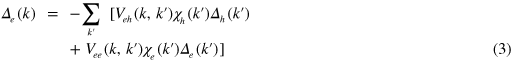
where  ,
,  , etc are the interactions defined in equation (1). For the convenience of the analysis of
  , we introduced the FS averaged pairing potential
  , etc and the coupled
  -equations are written as
where the pair susceptibility is defined as

and  are the density of states (DOS) of the hole band and electron band, respectively. For simplicity of demonstrating the mechanism, we temporarily drop the intra-band interactions
  and
and  , which are always much weaker than
  . Then the
  -equations can easily be combined to be


hence we can read off the critical temperature as

with  . Now if the electron band does not cross the Fermi level and the bottom of the band is lifted above the Fermi level by
  , the only modification of the above analysis is to replace the susceptibility of the electron band as follows

and the coupled  -equation, equation (7), changes as follows

The critical temperature is then reduced as

with ![${{\overset{}{\mathop{\lambda }}\,}_{eff}}=[{{\bar{V}}_{he}}{{N}_{e}}{{\bar{V}}_{eh}}{{N}_{h}}]\cdot \ln \left[ \frac{1.14{{\Lambda }_{hi}}}{{{\epsilon }_{b}}} \right]$](https://content.cld.iop.org/journals/1367-2630/16/2/023029/revision1/njp488374ieqn47.gif) . Notice that this analysis is accurate only when
. Notice that this analysis is accurate only when  , and in the other limit the susceptibility
  of equation (9) should be numerically calculated. Nevertheless, this simplified analysis clearly demonstrates the fact that in the multiband pairing model, where the main pairing interaction is the inter-band scattering, the FS instability still operates even if the FS of the electron band disappears and the
  will continuously decrease as the bottom of the electron band
  is lifted up above the Fermi level.
In figure 1, we show the numerical results of  calculated with equation (4) and the pair susceptibilities equations (5) and (9) numerically calculated. We also include both interband (
 and
and  ) and intraband (
 and
and  ) interactions. The FS averaged interaction can still be defined when the FS of the electron band disappears, for example, as follows
where the high energy cut-off  can be understood to be the high energy cut-off of the AFM spin fluctuations mediated pairing interaction
  . The above formula explicitly shows that the pairing interaction exists as far as
  and its strength only depends on the average distance of the momenta
  and
and  . The effective pairing interaction, of course, is proportional to the volume of the phase space connected by the interaction as

and this information is absorbed in the definition of the pair susceptibility (equation (9)) and  , the average DOS of the electron band in the region of
  , is a constant to a good approximation because the band dispersion
  is a quasi-2-dimensional parabolic band near the bottom of the band.

Figure 1. Numerically calculated  of the two band model vs the bottom of the electron band
  for different values of the intra-band interaction
  and
and  .
.  values are normalized by
  . We assumed a repulsive interaction for
  but considered both repulsive and attractive interactions for
  . For simplicity but without loss of generality, we also chose
  and
and  .
.
Download figure:
Standard image High-resolution imageThe above defined repulsive inter-band interaction  will induce the
  gap solution [8] and its precise value need not be specified because the final results are normalized as
  vs.
vs.  in figure 1. Also, instead of using the actual values of the intra-band interactions
  ,
,  , we treat them as free parameters for the purpose of demonstration. With this freedom and for generality, we considered both repulsive and attractive intra-band interaction in figure 1; the attractive intra-band interaction can possibly be caused by phonons [16]. When the intra-band interaction
  is sufficiently attractive (the case
  in figure 1, for example), the
  finally converges to the limit where only the hole band develops a SC transition with the attractive interaction. The gap symmetry does not change in this evolution because it evolves as
  with
with  .
.
In figure 1, we show the calculations starting from the negative value of  , which means that the electron band sinks slightly below the Fermi level and hence has a small FS. The positive
  value means that the bottom of electron band is lifted above the Fermi level by
  . The overall behavior of
  in figure 1 is similar for all cases; a linear decrease for small
  value and then exponential decrease for large
  value in accord with equation (11). This behavior is in qualitative agreement with the experimental observation of
  variation of
  compound with K doping [10–12, 14]. It should be desirable to have a good estimate of the model parameter
  vs. the K-doping x. Sato et al [5] found that the band structures of
  and
and  are pretty well matched by a rigid band model and the chemical-potential shift of 20–25 meV. They also estimated
  , hence we estimate
  –7 meV. However, in the real system, the K-doping will not only lift the electron band but also cause many other changes such as the hole FS sizes, the spin fluctuations strength, etc. Nevertheless, our calculations of figure 1 strongly suggest that the continuous lifting of the bottom of the electron band with K-doping (x) and its distance
  from
from  can be the leading factor for controlling
  in the
  compound. This pairing state in the lifted or sunken band close to the Fermi level was also considered in previous works [9, 13], but there the systematic investigations for understanding the phase diagram and other physical signatures were not carried out. Finally, during the calculations of figure 1, we assumed that the pairing symmetry maintains the same pairing state
  . In section 4, we will show that this is the most natural, and also consistent, assumption.
3. The shadow gap in the electron band
Here we solve the coupled gap equations, equations (2) and (3), for  with the realistic tight binding bands [8] and the fully momentum dependent phenomenological pairing interaction of equation (1). We used two model bands:
  and
and  with the band parameters as (0.30, 0.24, −0.6) for the hole band and (1.14, 0.74,
  ) for the electron band with the notation (
 ). The electron band located in the M points (
 in the folded BZ) is artificially lifted by shifting the parameter
  . The overall pairing strength
  (equation (1)) need not be physically accurate since all results are normalized by the gap values.
In figure 2, we show the calculated DOSs,  ,
,  , and the total
  . Figure 2(A) is the case when
  . In the normal state, the electron band and its DOS
  exists only above the Fermi level. Nevertheless, in the SC state, the Bogoliubov quasiparticles are formed above and below the Fermi level, hence the DOS
  is created both for
  and for
  . However, the shape of
  is very asymmetric for above and below
  as seen in the right inset of figure 2(A). It should be contrasted with
  in the left inset which is symmetrical, as a typical SC DOS. The total DOS,
  , displays this clear signature of the asymmetric DOS due to the electron band above the Fermi level. Figure 2(B) is the case
  . In this case the gap size in
  becomes
  and the shapes of
  and
and  become even more asymmetric than the
  case. This predicted asymmetric DOS could be detected by STM or tunneling measurements although the multiple peaks due to the multiband nature of the Fe-based superconducting compounds might obscure a clear separation of the predicted asymmetric DOS due to the shadow gap from other features. However, next we predict that a more direct and unambiguous signature of the shadow gap can be measured in the ARPES experiment.

Figure 2. Calculated density of states of each band,  ,
,  , and the total
  of the two band model in the SC state. (A) is the case of
  and (B) is the case of
  .
.
Download figure:
Standard image High-resolution imageIn figure 3, we showed the quasiparticle spectral density of the electron band near the M point. This is calculated by ![$\frac{1}{\pi }Im{{G}_{e}}(\omega ,k)=\frac{1}{\pi }Im\frac{\omega +{{\epsilon }_{e}}(k)}{{{\omega }^{2}}-[\epsilon _{e}^{2}(k)+\Delta _{e}^{2}]}$](https://content.cld.iop.org/journals/1367-2630/16/2/023029/revision1/njp488374ieqn135.gif) . These results are another manifestation of the shadow gap feature of the electron band which does not have FS. Figures 3(A) and (B) are the normal state and the SC state of the case
. These results are another manifestation of the shadow gap feature of the electron band which does not have FS. Figures 3(A) and (B) are the normal state and the SC state of the case  , respectively, and figures 3(C) and (D) are the corresponding results of the case
  . In the normal state, the quasiparticles do not appear below the Fermi level both in figures 3(A) and (C) simply because the band does not exist there. However, when temperature decreases below
  , the quasiparticle spectral density appears below the Fermi level both in figures 3(B) and (D). This shadow band behavior should appear only when the lifted electron band—hence having no FS pocket—participates in pairing of the
  gap state, otherwise it would not. This dramatic effect should be easy to detect by the ARPES measurement and in fact it seems to have already been detected in the
  compound by Shin and coworkers [17] although there the lifted electron band (about
  above
above  ) occurs at the
  point and these authors' interpretation is different from ours.

Figure 3. The quasiparticle spectral density of the electron band  near the M point. (A) and (B) are the normal and SC state, respectively, of the case
  . (C) and (D) are the corresponding results of the case
  .
.
Download figure:
Standard image High-resolution image4. Evolution of a nodal gap in

 , the end member of
  with x = 1, has been considered the strongest candidate for a nodal gap superconductor among the iron-based superconductors [18–21]. However, the optimal doped
  compound is confirmed to have isotropic full s-wave gaps [3]. Therefore, the evolution from a full gap to a nodal gap in the
  compound has been of great interest over the years [10–12, 14, 22].
In this section, in order to study the gap evolution in  , we introduce the minimal three band model. We added one more hole band (
 ) around the
  point,
  , to the two band model introduced in the previous section, so that we have two hole bands
  and
and  and one electron band e. The second hole band
  is tuned to have a larger FS than the
  hole band; we used parameters
  and varied
  . With K doping, the FS sizes of both
  - and
- and  - bands will increase but the FS of the e-band will decrease and then disappear for
  –0.7. The spin fluctuations will also change with K doping; the neutron scattering study of [14] showed that the strong and well defined spin fluctuations continue to exist up to
  but develops the incommensurability of
  with
with  while the optimal doped
  has
has  Its overall strength will also change.
However, our intention in this section is to focus on and investigate the correlation between the FS size and the anisotropic or nodal gap evolution in the most clear manner and therefore we ignore the above mentioned changes of the real system except the FS size variation. Further, because we have already shown in the previous section that the main hole band ( ) and the electron band (e)—whether it has a FS or not—maintain the
  -pairing state via the inter-band repulsive interaction, we also fix the FSs of the
  and e bands and only vary the FS size of the
  band. The spin fluctuation interaction
  given by equation (1) is also fixed with
  and
and  [15] for all calculations. Therefore, our model calculations in this section should be considered a theoretical experiment designed for revealing the possible role of the FS size of a hole band for developing a nodal gap when all other conditions are fixed.
We have solved the coupled gap equations with three bands, generalizing equations (2) and (3) by adding one more band to them, with the interaction potential  of equation (1) as inter-band and intra-band interactions among all three bands. We didn't impose any constraint on the shapes and signs of the gap functions
  except
  symmetry. In figure 4, we showed the gap solutions for the several different sizes of the
  -hole pocket. In the left panel, the FSs of three bands are drawn for different values of
  in the folded BZ. In the case of e-band, a tiny e-band pocket is drawn only for indication but in real calculations its size was chosen to be zero with
  . As expected, when the
  -hole pocket and the
  -hole pocket have similar sizes as in figure 4(A), the corresponding gap solution shown in the right panel is basically a
  s-wave state with some anisotropy. The reason why the
  gap has the same sign as the
  gap is simply because the average distance between the
  -FS and the e-FS is closer to the AFM peak momentum
  than the distance between the
  -FS and the
  -FS to
  . Increasing the
  -FS size in figure 4(B), these distances become comparable (including the weighting factors of the DOSs,
  ,
,  and
and  ) so that the inter-band interaction from the
  -band (which tends to develop a
  gap on the
  -band) and the inter-band interaction from the e-band (which tends to develop a
  gap on the
  -band) almost cancel each other out on the
  -FS. As a result, the gap size of
  becomes vanishingly small as seen in figure 4(B). Although this happens with a fine tuning of the FS size of the
  -band in our model calculation, this vanishingly small gap should naturally occur as a horizontally vanishing gap—like a horizontal line node—when the FS size continuously increases along the
  -direction, as observed in the
  -band of
  by ARPES measurement [23].

Figure 4. (left panel) The FS evolution of the three band model ((A)–(D)); only the  -FS (green line) size varies in the whole calculation. Also the e-FS (blue line) is shown only for indication and in real calculations it has zero size by choosing
  . The pink line is the magnetic BZ as a guide for the eyes. (right panel) The corresponding gap solutions
  (red line),
  (green line), and
  (blue line), respectively. The Fermi surface angle is measured from the x-axis.
Download figure:
Standard image High-resolution imageFurther increasing the  -FS in figure 4(C), both the
  -band (
 gap) and the e-band (
 gap) exert similar strength but opposite pairing interactions on the
  -band which do not exactly cancel out at each point of the
  -FS. Therefore the
  -band maximizes the condensation energy gain by mixing
  gap and
  gap on the different sections of the
  -FS, hence developing accidental nodes but keeping
  symmetry because of the
  crystal symmetry. Increasing the
  -FS size even further in figure 4(D), the average distance between the
  -pocket and the
  -pocket increases and therefore the repulsive interaction from the
  -pocket also increases, hence
  develops more negative lobes.
Figure 5 shows the same calculations as in figure 4 but choosing a finite value  , hence the electron pockets are completely lifted above the Fermi level. A choice of this value
  is to simulate the fully doped
  . According to Sato et al [5],
  of
of  was roughly estimated to be 2–7 meV, so we assumed it to be
  and the spin fluctuation energy scale
  . We emphasize that these values are not intended to be precise but only to give some ball-park guideline.

Figure 5. The same calculations as in figure 4, except choosing  . Hence the electron band is lifted above the Fermi level by
  and the electron pockets have completely vanished in the left panel. Notice, however, that the electron band still forms a gap solution
  as shown in the left panel.
Download figure:
Standard image High-resolution imageAs explained in section 2, the main change caused by increasing the  value is the reduction of the pair susceptibility of the electron band
 ![${{\chi }_{e}}({{\epsilon }_{b}})\approx \ln \left[ \frac{1.14{{\Lambda }_{hi}}}{{{\epsilon }_{b}}} \right]$](https://content.cld.iop.org/journals/1367-2630/16/2/023029/revision1/njp488374ieqn241.gif) . As a consequence, the effective repulsive interactions exserted from the e-band onto the
. As a consequence, the effective repulsive interactions exserted from the e-band onto the  - and
- and  -pockets become weakened, and the other conditions are almost the same as in figure 4. Therefore, the evolution of the gap solutions from (A) to (D) is qualitatively similar to the case of figure 4 but we notice two quantitative changes: (1) the overall gap sizes (
 , and
, and  ) are reduced because of the weakened pair susceptibility
  ; (2) the negative portion of the
  gap function relatively increases again because the effective repulsion from the electron band—which itself forms a negative sign gap (
 )—becomes weakened. For example, comparing figure 4(B) and figure 5(B), a tiny positive
  in figure 4(B) becomes a nodal gap
  with a mixture of tiny positive and negative portions in figure 5(B). Similarly, the magnitudes—relative magnitudes to the average gap size of each case—of the negative lobes of
  in figures 5(C) and (D) become bigger than the ones in figures 4(C) and (D), respectively.
In our simple model, the pairing interaction equation (1) is oversimplified and even orbital degrees of freedom is completely ignored, therefore our gap solution results cannot be quantitatively compared to the real compounds. However, this dramatic gap evolution with only a small variation of the FS size demonstrates that the subtle balance of the inter-band repulsive interactions between bands can be the crucial mechanism for developing and stabilizing the nodal gap solution
1
. In this regard, the most important role is still played by the hidden electron band. Although its FS disappears, the e-band develops the largest gap  (see the right panel in figure 4)—which is the inevitable consequence of the interband paring mechanism (
 ) [8]—and therefore this hidden e-band, although lifted above the Fermi level, continues to play the important role of balancing the overall
  gap state and inducing a nodal gap on the
  -band with a larger FS. Finally, if we consider that the
  -pocket in our model corresponds to the outer or middle hole pocket of
  , the overall gap anisotropy of
  and its systematic development of the nodal gap structure is surprisingly similar to the recent ARPES measurements on
  with K doping by Shin and coworkers [14, 24]. As has been repeatedly stated, quantitative comparisons such as the magnitude of the gap sizes with doping etc should not be done using our model calculations.
5. Conclusion
We showed that the absence of a FS does not prohibit FS instability of the SC transition in the multi-band model mediated by inter-band pairing interaction. Although we used a simplified model calculation ignoring realistic details, it is a proof of principle. Applying this pairing mechanism with a missing FS to the two band model where the electron band is lifted up by  above the Fermi level, we also showed that the
  evolution vs.
  qualitatively captures the experimental
  evolution of
  with K doping. As proof that our scenario forms the SC gap in the hidden electron band, we predicted the shadow gap features using both ARPES and tunneling measurements, which can be easily tested experimentally. Finally, we demonstrated that the presence of the hidden electron band plays a crucial role in developing a nodal gap on the larger hole pocket (
 ) in the three band pairing model. This result might contribute to the understanding of nodal gap development in
  [14, 24] as well as
  [23] compounds.
Acknowledgments
This work was supported by grant nos. NRF-2011-0017079 and 2013-R1A1A2-057535, funded by the National Research Foundation of Korea.
Footnotes
- 1
The intra-band repulsive interaction
also contributes but it mainly shifts the balance in the parameter space. When the -FS size becomes very large, the intra-band interaction itself tends to drive a d-wave nodal gap rather than the -nodal gap as found here.


