


Abstract
We discuss a two-color SASE free-electron laser (FEL) amplifier where the time and energy separation of two separated radiation pulses are controlled by manipulation of the electron beam phase space. Two electron beamlets with adjustable time and energy spacing are generated in an RF photo-injector illuminating the cathode with a comb-like laser pulse followed by RF compression in the linear accelerator. We review the electron beam manipulation technique to generate bunches with time and energy properties suitable for driving two-color FEL radiation. Experimental measurements at the SPARC-LAB facility illustrate the flexibility of the scheme for the generation of two-color FEL spectra.
Export citation and abstract BibTeX RIS

Content from this work may be used under the terms of the Creative Commons Attribution 3.0 licence. Any further distribution of this work must maintain attribution to the author(s) and the title of the work, journal citation and DOI.
GENERAL SCIENTIFIC SUMMARY Introduction and background. Free-electron lasers (FELs) are demanding for advanced photon science experiments thanks to their properties in terms of transverse coherence and flux in a narrow bandwidth wavelength. The FEL process is driven by high brightness electron beams whose energy is the main knob for tuning the wavelength of FEL radiation. The ability of FELs in the x-rays range to probe matter at the femtosecond time scales is typically exploited in pump–probe configurations where two pulses with different wavelengths and adjustable time delay are used to investigate the processes occurring during chemical and physical reactions. One method, exploited at SPARC-LAB, to generate two-color FEL radiation consists in injecting in the undulator a train of two electron bunches with time and energy separation adjustable by setting the linear accelerator (linac) parameters.
Main results. A two level electron beam energy distribution has been produced to maximize the frequency and time separation ranges of the FEL radiation, resulting in lasing from two separated and nearly independent electron distributions. The electron parameters and thus the radiation time and frequency separation can be tuned by adjusting the accelerator working point. The total radiation bandwidth is set by the electron energy separation and not by the FEL parameters, further reducing the light pulse duration.
Wider implications. To overcome the intrinsic FEL fluctuations coming from shot-noise, our method can be extended to seeded FEL schemes, where the emission is locked to an external seed laser.
 Figure. Schematic layout of the SPARC photo-injector. The ensemble of electron beam time and energy configurations at the linac exit for three different longitudinal compression regimes.
1. Introduction
The success of x-ray free-electron lasers (XFELs) arises from the unprecedented characteristics of the photon beams such as extremely large peak power, very short pulse duration and ultra high peak brightness electron beams [1, 2]. Depending on the experimental application, large flexibility in the x-ray pulse shape and parameters is required, and the demands of fourth generation x-ray users continuously push the limits and increase the variety of designs and performance of current and future light sources.
The ability of XFELs to probe matter at the ultrafast time scales is typically exploited in pump–probe configurations where two pulses with different wavelengths and adjustable time delay are used to investigate the processes occurring during chemical and physical reactions [3–6]. A first pulse, the pump, is used to deposit an initial excitation energy into the system and initiate a reaction; a second pulse, the probe, is then used to both sample the state of the reaction after a certain time delay, and detect the event. By varying the time delay between pump and probe, and observing the response of the sample, a movie of the ultrafast process under study can be reconstructed [7]. In the most common configuration, an optical laser is used for pumping and the x-rays for probing the system, but some systems require pump photons with higher energy. For these experiments, the option of using two short wavelength pulses with adjustable temporal separation is attractive. Optical schemes to split and delay the photon beam have already been successfully used with XFELs [8, 9], but mostly require Fourier transform holography to distinguish the frame on an integrating slow-detector [10]. Frequency separation might be desired in this case to allow clear distinction of the probe signal. With a second independently tunable frequency it would also be possible to tune into hardly accessible states of the system and follow the flow of energy into initially unexcited states. Other interesting applications of two-color x-ray pulses profit from the extra information contained in the multi-wavelength spectrum in coherent diffractive imaging techniques [11], or are related to differential imaging when the central wavelength is tuned close to an absorption edge of the sample.
Various schemes for generating two colors from a FEL amplifier have been proposed, with the first papers dating back more than 20 years, in a period when optical parametric amplifiers were not commercially available and even the tunability offered by FELs at infrared and visible wavelengths was a unique feature. The main advantages of a two-color FEL, with respect to two independent FEL beamlines, are simplicity and versatility, deriving from re-using the same hardware, and the minimization of the timing jitter between the two different pulses. To allow jitter-free FEL-pump/FEL-probe experiments, seeded FEL schemes [12], as recently demonstrated at the FERMI soft x-ray FEL, involve the use of either a chirped or a two-color seed laser which initiates the FEL instability at two different wavelengths within the modulator gain bandwidth [13–16].
Another option consists of the use of staggered undulator magnets having different values of K to achieve lasing at two distinct wavelengths [17, 18]. Recently at LCLS this idea has been revisited and the emittance-spoiler technique with a magnetic chicane in the undulator section was used to control the pulse duration and relative delay of a two-color intense x-ray pulse generated using two separate canted pole undulators tuned at different resonances [19]. The length of the FEL undulator in this case is essentially doubled, and a complex scheme is required to reach saturation and power levels comparable with the single color configuration.
A different approach is to inject in the FEL undulator a multi-energy electron beam in order to maximize the frequency and time separation ranges of the FEL radiation, while still maintaining similar saturated power levels and minimal undulator length [20]. In this configuration, the SASE lasing occurs from separated and nearly independent electron distributions.
For a relative electron energy separation  , the resulting radiation is characterized by a relative wavelength separation
  . Though a large beam energy spread usually degrades the performance of the FEL amplifier, when two narrow bandwidth energy distributions are injected in the undulator, appreciable FEL gain can be obtained at two separate wavelengths. In fact, if the two electron bunches have an energy separation larger than the FEL natural bandwidth (i.e.
  , or
, or  until saturation, ρ being the Pierce parameter [21]), regardless of their relative delay, the system will behave as two completely independent FELs without any gain competition [22]. Furthermore, if each beamlet length
  is smaller than
  , being
  , the cooperation length of the radiation, then the two pulses are characterized by single longitudinal modes.
A method for producing trains of electron bunches with sub-picosecond length, sub-picosecond spacing and adjustable time and energy separation has been developed and demonstrated [23, 25, 26] at the SPARC-LAB [27] test facility at LNF (INFN). The method is based on the RF compression of a beam generated from a photocathode illuminated by a comb-like laser pulse as reviewed in section 2.
In the present paper, we describe the proof of principle experiment concerning two-color SASE FEL lasing from two electron bunches with adjustable time delay and energy separation. Section 2 reports the method and, through numerical simulation, it highlights peculiar accelerator working points suitable for the production of different radiation patterns. Section 3 assesses our scheme reporting on the experiment held at SPARC-LAB: a full characterization of the driving electron bunches as well as of the FEL radiation is presented. Finally we will close with comments and conclusions.
2. Generation and control of two pulses with arbitrary temporal and energy separation
The method used at SPARC-LAB for tailoring an adjustable train of electron bunches, with sub-picosecond length and picosecond spacing, combines UV laser pulse shaping and low-energy electron beam longitudinal compression techniques, namely the laser comb and the velocity bunching, respectively.
Section 2.1 describes the generation of the comb laser beam at SPARC-LAB, with reference to the different schemes adopted elsewhere, while section 2.2 discusses the generation and manipulation of the bunch trains focusing on the two pulse electron bunches relevant for this manuscript. Measurement results showing the flexibility of the proposed scheme are eventually reported in section 2.3. Further details on the velocity bunching technique and how it is implemented at SPARC-LAB can be found in [28, 29] and related references, as well as a complete SPARC linac description.
2.1. Generation of a comb laser beam
A comb laser beam is characterized by two or more short (hundreds of fs) pulses spaced by a few picoseconds. The technique, used at SPARC-LAB for the experiment presented here, relies on a birefringent crystal, where the input pulse is decomposed in two orthogonally polarized pulses with a time separation proportional to the crystal length,  , as given by
  ;
;  and
and  are, respectively, the ordinary and extraordinary indexes of refraction at the wavelength of 266 nm, and c the speed of light. The crystal is α-cut beta barium borate (BBO), which is a UV transparent optical material characterized by a strong birefringence. The α-BBO crystals are oriented with fast and slow axes at
  with respect to the incident horizontal polarization, so that a single pulse is equally split into two pulses, with the orthogonal polarizations traveling at different group velocities. Since the crystal has its optical axis parallel to the front surfaces, there is no spatial walk-off between the ordinary and extraordinary beams, and the output pulses are naturally aligned. If more birefringent glasses are inserted in the laser beam path, it is possible to produce multi-peaked laser pulses [30, 31].
A completely different approach to produce picosecond-spaced bunch trains consists of placing a mask in a high dispersion, low beta function region of a dogleg beam line in order to produce a temporal bunch train out of a long bunch with a correlated energy spread. The bunch train structure is very stable in time and energy because the mask is a fixed object in a dispersive section of a beam line; the drawback is that approximately 50% of the initial charge is lost in such a process ([32] and related references).
For the measurements reported in this paper, short (150 fs FWHM) UV pulses were sent to a birefringent crystal of 5.49 mm length, in order to induce a time separation  = 4.27 ps. The birefringent material is coated with an antireflection layer, and the energy losses can be limited to a few percent. In addition, to change the relative intensity of the two pulses, a half-wave plate is inserted before the α-BBO. This feature allows us to control the charge emitted by the two pulses and to compensate for the variation in the quantum efficiency due to different gun extraction phases for the two pulses. After the birefringent crystal, a variable neutral density filter is used to reduce the overall energy. For the present experiment, the total energy was in the tens of μJ range. Interested readers can find additional details in [23].
In this technique, the time separation at the cathode is set by the crystal length and cannot be easily changed. Therefore the time separation of the two bunches at the linac exit can be controlled by manipulating the electron beam longitudinal phase space under proper operation of the linac, as described in the following subsection.
2.2. Train of electron pulses from a comb laser beam
The SPARC linac layout is schematically sketched in figure 1. The linac consists of a 1.6 cell S-band (2.856 GHz) RF gun with a peak field of  followed by three SLAC type 3 m long traveling wave (TW) sections which in the rest of the paper we refer as S1, S2 and S3. Downstream of the third accelerating section, a diagnostic line is placed including a five-cell standing wave RF deflecting structure, that combined with the dipole magnet is used to reconstruct the longitudinal phase space by analyzing the beam image on a scintillating screen.
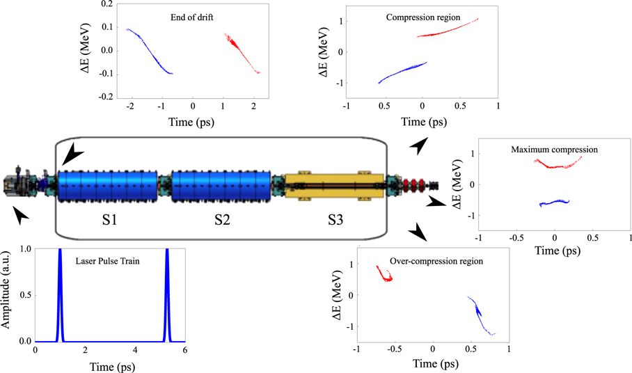
Figure 1. Schematic layout of the SPARC photoinjector. The evolution of the electron beam longitudinal phase space along the linac is depicted in the insets for three different RF compression phases, together with a comb laser pulse profile generating the comb electron beam distribution (GPT simulation [24], total bunch charge 160 pC, laser pulse separation 4.27 ps).
Download figure:
Standard image High-resolution imageThe comb laser pulse (figure 1) illuminates the copper photocathode embedded in the RF gun, and it generates a train of short electron bunches with the same pulse distance. The beam, accelerated to an energy of about 5.8 MeV in the RF gun, is then injected in the first linac section S1. In the drift downstream of the RF gun, the beamlets undergo a broadening due to space charge effects with a correspondent energy modulation. Then, a dispersive section, i.e. S1 working as an RF compressor, will act on the density modulation, producing a beam with time separation depending on the S1 compression phase. The insets in figure 1 depict a GPT simulation, showing the evolution of the comb electron beam longitudinal phase space at the end of the drift and for three different RF compression phases.
The main knobs used to tune the final beam distribution in the longitudinal phase space are the phases of the first (S1) and third linac (S3) section. Moving along the velocity bunching compression curve and properly choosing the linac set points, it is possible to obtain two beamlets with different energy and time separations. Careful tuning of the accelerator is required to move from one working point to another.
Experimental results with a two-bunch train as generated and characterized at SPARC-LAB for different applications are reported in [33–35]. Typical values of the total bunch charge range from 70 to 180 pC with an energy from 160 to 110 MeV, depending on the injection phase in the RF compressor.
In the following we will refer to the TW section phases with respect to the maximum energy (on crest) case; thus in this manuscript an S1 phase of  means that the beam injection phase in the first TW section is
  away from the on crest phase. The same convention applies to all the TW section phases.
An example of what happens when the S1 phase is varied is shown in figure 2. The plot in the upper box of figure 2 reports the compression factor, defined as the ratio between the bunch length on crest and the bunch length after compression, while the plot in the lower box depicts the total bunch length and the distance between the two pulses, both as function of the S1 phase, as computed by TSTEP simulations [36].
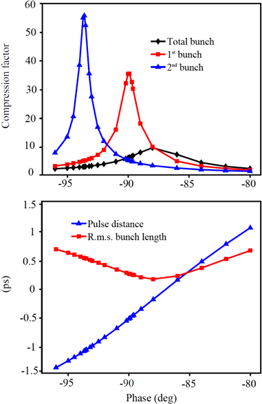
Figure 2. Upper box: compression curves for the total beam and single pulses. Lower box: computed bunch length and two pulse separation versus the S1 phase (TSTEP simulation, total bunch charge 165 pC, laser pulse separation 4.27 ps).
Download figure:
Standard image High-resolution imageMoving the S1 phase from the crest towards the zero crossing of the RF field (i.e. moving leftwards in figure 2, upper box), the maximum bunch compression is reached. Moving further brings the beam to over-compression where the whole bunch starts lengthening. The single sub-bunches reach their maximum compression for more negative values of the S1 phase with respect to the total beam, which means that only in the over-compression region are the two bunches actually well separated in time. The pulse inter-distance spans the sub-picosecond range (figure 2, lower box), with the negative sign on this curve corresponding to the longitudinal over-focusing condition in which a head–tail interchange between the two pulses occurs.
Extensive computer simulations have been performed to investigate the dependence of the tuning range of the two bunch distance on charge and laser pulse separation at the cathode ( ). Figure 3 shows the pulse inter-distance as a function of the S1 phase; the slope of the curve increases with
  and/or the total charge.
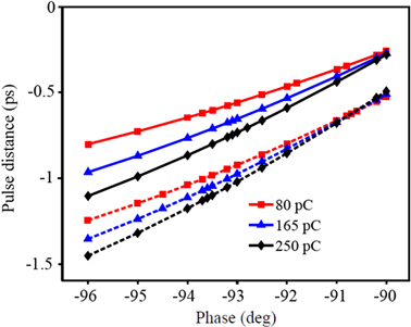
Figure 3. Computed tunability curves of two-pulse separation in different operating conditions in the over-compression region for laser pulse separation of  (solid lines) and
  (dashed lines) (TSTEP simulation).
Download figure:
Standard image High-resolution imageThe temporal structure is almost frozen at the exit of S1 where the beam is compressed and accelerated, so the phase of the following sections (i.e. S2 and S3) can be used as an independent knob to control the final energy separation between the two bunches. An example of the energy separation dynamics is presented in figure 4, showing how the energy separation can be easily tuned by moving the S3 phase without changing the pulse inter-distance (fixed by the S1 phase value).
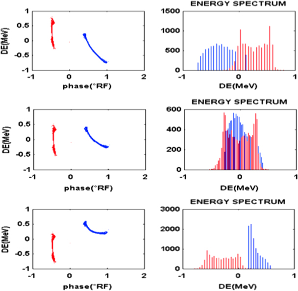
Figure 4. Longitudinal phase space and energy distribution versus S3 phase:  (top),
  (middle),
  (bottom) (TSTEP simulation, total bunch charge 165 pC, laser pulse separation 4.27 ps).
Download figure:
Standard image High-resolution imageTo summarize, we can conclude that the bunch inter-distance is mostly affected by the S1 phase, while the energy separation is mainly tuned acting on the S3 phase. The second section usually works on crest, but the phase on S2 can also be moved for fine tuning of the energy spread of single pulses. Besides, the machine working point is affected by the laser pulse separation (i.e. the α-BBO crystal length in the SPARC scheme), the bunch charge as well as the gun injection phase; all those parameters are used to finely tune the machine working point.
2.3. Measurements
The tuning capability of the system has been verified experimentally by reconstructing the longitudinal phase space at the linac exit with the use of the vertical deflecting cavity coupled with the horizontally dispersing dipole.
In practice, the following procedure is used to set up the machine. A laser pulse train made of two pulses, with an initial single pulse length of 150 fs and separated by 4.27 ps, is sent to the copper photocathode to generate a two-bunch train. The generated electron bunch train is injected in the gun at  , close to the phase of maximum energy, and on the crest of the RF field in S1 (
 , maximum energy): such a maximum energy configuration is used as a reference for machine operation and start-to-end simulations.
Then the phase of the first TW cavity (S1) is moved from the crest value to the phase of maximum compression ( ). At this phase the bunch train length achieves the minimum value corresponding to a full spatial overlapping of all the bunches with a typical total energy separation of about 1 MeV, and each electron pulse is also partially compressed.
By moving further in the over-compression regime (typically  off crest) one can obtain two pulses with tunable distance and fixed energy separation. In order to precisely control the temporal distance between the two pulses and keep it constant over time, the RF phase jitter of the velocity bunching section must be reduced to less than
  (rms) of the RF phase. This was obtained using intrapulse RF feedback and a closed-loop circuit of the water temperature stabilization. Afterwards, the phase of the third linac section can be used to fine tune the central energy as well as the energy separation of the two pulses.
In figure 5 the raw longitudinal phase space images are shown for three different working points: moderate bunch compression region (figure 5(a)), maximum compression point (figure 5(b)), and over-compression region (figure 5(c)).

Figure 5. Raw experimental images of the longitudinal phase space in three different working points: moderate bunch compression region (a), maximum compression point (b), over-compression region (c) (total bunch charge 165 pC, laser pulse separation 4.27 ps).
Download figure:
Standard image High-resolution imageIn the moderate compression (figure 5(a)) the two beamlets are partially overlapping in time, while being well separated in energy. On the contrary, in the maximum compression point the two bunches are fully superimposed in time, remaining with two distinct energy levels (figure 5(b)). Eventually with the over-compression, one can produce two bunches of the same energy but with different arrival times at the linac exit (figure 5(c)). Obviously all the intermediate conditions can be achieved with proper machine settings.
An automated image analysis tool has been developed to extract the important information from the raw longitudinal phase space images (total and single bunch length and energy) with a resolution of 50 fs in the bunch length measurements after deconvolution with the unstreaked spot size.
3. Two-pulse SASE FEL spectra
The method described in the previous section allows a relatively large tuning range of the time and frequency properties of the FEL emission suitable for a wide range of applications [5–7]. In particular, pump and probe experiments require an adjustable time delay between the two-color pump and probe pulses. An example of the double-peaked signature in both the spectrum and time of the SASE FEL radiation, as obtained through the method explained in the previous section, is reported in figure 6. The spectrogram of the two-color SASE FEL radiation, measured by means of a FROG device 8 , confirms the temporal separation of the two pulses.

Figure 6. Experimental (a) and retrieved (b) FROG traces in the case of a two-energy level, ps spaced two-bunch train. FROG temporal (c) and spectral (d) signal, showing the double-peaked structure both in frequency and time (total bunch charge 165 pC, laser pulse separation 4.27 ps).
Download figure:
Standard image High-resolution imageExperimental results in different configurations which give rise to unique FEL spatio-temporal features (beam overlapped in time or in energy) have already been presented elsewhere [20, 37].
In this section we extensively discuss experimental investigations on the SASE FEL spectral emission properties measured in the three working points summarized in table 1 (Cases A, B, C) and figure 7.
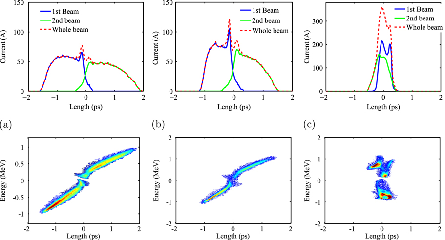
Figure 7. Current profile (upper row) and longitudinal phase space (lower row) measurements for three different S1 phases: (a)  E = 1.01 MeV,
  T = 1.39 ps; (b)
  E = 1.14 MeV,
  T = 1.01 ps; (c)
  E = 1.19 MeV,
  T = 0.1 ps.
Download figure:
Standard image High-resolution imageTable 1. SPARC linac parameters for comb-FEL emission centered at 800 nm.
| Case A | Case B | Case C | |
|---|---|---|---|
| Total charge | 160 pC | 160 pC | 180 pC |
| Phases S1/S2/S3 |

|

|

|
| Central beam energy | 85.916(0.020) MeV | 88.433(0.039) MeV | 88.098(0.101) MeV |
| Normalized projected emittance | 1.635(0.041) mm mrad | — | 3.88(0.13) mm mrad |
Undulator 
|
0.78 | 0.78 | 0.84 |
Figure 7(a) is the electron beam longitudinal phase space, corresponding to Case A, resulting in an energy separation of 1.011(0.033) MeV, peak current around 70 A and a distance between the maximum current peaks of 1.391(0.040) ps. In Case B, figure 7(b), the S1 phase is closer to the maximum compression point and the distance between the two pulses decreases down to 1.014(0.028) ps, while the energy separation increases to 1.136(0.062) MeV. Case C (figure 7(c)) concerns the maximum compression (S1 phase equal to  off crest), being characterized by the complete overlap in time of the two pulses and an energy separation of 1.191(0.046) MeV; the peak current approaches 200 A.
The transverse phase space is examined through a standard quadrupole scan technique to measure the total projected emittance reported in table 1 [38].
After an extensive characterization of both longitudinal and transverse parameters, the electron bunch train is injected in the six undulator modules with 77 periods (period length = 2.8 cm) interspaced by 30 cm separation where horizontally focusing quadrupoles are used to compensate the vertical natural focusing of the undulator. Transverse matching of the beam in the FODO lattice is done by tuning the two quadrupole triplets located before the undulator using the average Twiss parameters obtained from the emittance measurement. Though the resulting matching conditions are not ideal for any of the two beams which have slightly different energies and Twiss parameters, they appear to be transversely superimposed and lasing occurs for both sub-bunches, because the differences are at percent level.
Using the measured parameters, the estimated one-dimensional ρ parameter for each of the two beamlets is  . This quantity defines the FEL spectral bandwidth. For an energy separation of percent level, the difference in resonant frequencies makes the two pulses emit two separated spectral lines independently. Furthermore, since the total slippage is 300 fs and the pulses are shorter than a cooperation length (for instance around 150 fs rms), they radiate in a single-spike regime.
The output of the SASE FEL is characterized by two very distinct radiation spectra in good agreement with start-to-end simulations [20], performed with the GENESIS code [39]. Three representative single shot spectra corresponding to the longitudinal phase space cases described earlier are shown in figure 8. They have been measured using an Ocean Optics spectrometer with 1.2 nm resolution. The central frequency for all these cases is 800 nm. It should be noted that the separation between the spectral peaks remained constant during the data acquisition, but both the center frequency and the relative amplitude of the two peaks can vary due to machine and SASE process fluctuations. The single spike SASE regime is in fact characterized by 100% shot-to-shot fluctuations.

Figure 8. Single-shot two-color SASE FEL spectra for the three different working points of table 1.  is the central wavelength of the two peaked spectra. The spectrum of the radiation was measured using an Ocean Optics spectrometer with 1.2 nm resolution at 800 nm.
Download figure:
Standard image High-resolution imageAs the energy separation between the two electron beam distributions is changed, we observe a relative frequency distance between the pump and probe pulses up to 6%, a bandwidth almost one order of magnitude larger than any other two-color FEL experiment reported up to now. For example for case A having an energy separation of 1.01(0.03) MeV, the expected spectral separation is  in good agreement with the measurement shown in figure 8. The total energy in the radiation pulse was measured using a Joulemeter (Molectron J3-S, 5.96E8
  @ 1 μm) with the density filters, showing values consistently larger than 40–50 μJ. This observation, together with the spectral evidence of a significant second harmonics signal, indicates that the system is approaching saturation. It should be observed that the signal at the second harmonic also presents a two peaked spectrum, as depicted in figure 9 (lower box). Due to the wide bandwidth acceptance of the spectrometer, this spectrum is taken simultaneously to the fundamental spectrum reported in figure 9, upper box. The relative amplitude of the second harmonic is two orders of magnitude lower as predicted by simulations. The shape and relative separation of the peaks thus match the fundamental profile very well. The separation of the second harmonic peak is exactly half of the corresponding fundamental frequencies, as expected. This is the first evidence for two-color harmonic radiation in FELs.

Figure 9. Fundamental (upper box) and second harmonic (lower box) single-shot measured spectra from the double-peaked energy distribution (total bunch charge 165 pC, laser pulse separation 4.27 ps).
Download figure:
Standard image High-resolution image
4. Conclusion
The use of a two energy level electron beam for producing two-color radiation pulses has been studied and tested for the first time at SPARC-LAB. We have presented a technique relying on low energy RF compression of a comb-like electron beam, to produce high brightness, sub-picosecond spaced trains of pulses, separated both in energy and time, and capable of producing FEL radiation. Numerical simulations of the beam dynamics have pointed out the main parameters to achieve the desired beam properties in this two-bunch regime, demonstrating the versatility of the method. A specific case has been investigated in an experiment where the spectral and temporal features of SASE FEL radiation have been fully characterized; the results agreed very well with the simulations of both the electron beam dynamics and the FEL process. Our studies give a first insight into the color tunability of the pump and probe pulses that may be obtained with the proposed method.
Footnotes
- 8
FROG near-infrared GRENOUILLE: time-bandwidth product <10 spectral resolution 0.7 nm at 800 nm; single-shot sensitivity 1 μJ.