


Abstract
Amoeboidal cell crawling on solid substrates is characterized by protrusions that seemingly appear randomly along the cell periphery and drive the cell forward. For many cell types, it is known that the protrusions result from polymerization of the actin cytoskeleton. However, little is known about how the formation of protrusions is triggered and whether the appearance of subsequent protrusions is coordinated. Recently, the spontaneous formation of actin-polymerization waves was observed. These waves have been proposed to orchestrate the cytoskeletal dynamics during cell crawling. Here, we study the impact of cytoskeletal polymerization waves on cell migration using a phase-field approach. In addition to directionally moving cells, we find states reminiscent of amoeboidal cell crawling. In this framework, new protrusions are seen to emerge from a nucleation process, generating spiral actin waves in the cell interior. Nucleation of new spirals does not require noise, but occurs in a state that is apparently displaying spatio-temporal chaos.
Export citation and abstract BibTeX RIS

Content from this work may be used under the terms of the Creative Commons Attribution 3.0 licence. Any further distribution of this work must maintain attribution to the author(s) and the title of the work, journal citation and DOI.
1. Introduction
Many eukaryotic cells can crawl on solid substrates, for example, to move towards nutrients or other cells, to avoid toxins, or in response to other external stimuli [1]. Depending on the cell type and environmental conditions, several distinct types of cell crawling can be identified. Two extreme examples are provided by fish keratocytes that essentially maintain their shape and move directionally [2], and by the slime mold Dictyostelium discoideum or human neutrophils that display an irregular crawling via the formation and retraction of protrusions (pseudopods). The irregular pattern of motion is called amoeboidal movement and has been studied notably in the context of chemotaxis [3].
These different kinds of cell crawling rely on the same molecular machinery, namely, the actin cytoskeleton, which is a network of structurally polar, filamentous protein aggregates. For some cell types, it is known that the polymerization of actin filaments pushes the leading edge forward and thus provides the machinery of cell crawling [4]. In other cell types, the motor-induced contraction of the actin cytoskeleton squeezes the intracellular fluid, which in turn leads to the extension of a protrusion [5] and has been recently analyzed from a theoretical point of view [6–8]. However, it is largely unknown how the assembly of the actin network and its contractility is regulated on a cellular scale to achieve the crawling patterns observed in living cells, in particular, amoeboidal crawling.
Actin assembly can be regulated through external cues. For example, the direction of motion of a crawling cell can be controlled by an external gradient. Notably, chemical gradients are read out by cells able to perform chemotaxis. Remarkably, though, many eukaryotic cells and even cell fragments can also spontaneously polarize and choose a direction of motion [9–12]. Furthermore, some cells actively search for other cells by performing a random walk type of movement that is largely independent of external stimuli. Whereas mechanisms for this random cell motion have not been studied systematically so far, some ideas exist about how the cells can spontaneously polarize [13]. In particular, it has been suggested that cytoskeletal polymerization waves could play an important role in this context [14, 15].
Polymerization waves can emerge spontaneously from the interaction of actin filaments and nucleation promoting factors (NPFs) [14, 16–19]. Actin assembly is a process depending on the release of chemical energy through the hydrolysis of adenosine triphosphate (ATP). Opposite ends of actin filaments differ in their assembly kinetics, with the so-called barbed end usually growing on average, whereas the so-called pointed end typically shrinks on average, a phenomenon called treadmilling [20, 21]. Depending on the presence of other proteins, either shrinking at the pointed or growth at the barbed end can be faster. Under certain conditions, the system can also self-organize into a state where both rates are equal [22].
The pool of actin filaments is constantly turning over and disassembled filaments are replaced. Under physiological conditions, actin monomers do not assemble spontaneously to form the nucleus of a nascent filament. To this end, NPFs like the Arp2/3 complex or members of the formin family are used in cells. The Arp2/3 complex binds to an existing actin filament and then stays attached to the pointed end of the newly created actin filament. In contrast, formins stay attached for some time to the barbed end of the newly generated actin filament and assist elongation. If there is a negative feedback from existing filaments on active NPFs, for which some experimental evidence exists [14], then polymerization waves can emerge spontaneously [14, 17–19].
In this work, we study the consequences of spontaneous cytoskeletal polymerization waves on the migration of cells adhering to a substrate and in the absence of molecular motors. Indeed, it has been shown that mutants of D. discoideum lacking the molecular motor myosin II can still crawl on solid substrates [23]. Similarly, neutrophils crawl on weakly adhesive substrates in the presence of ML-9, an inhibitor of the myosin light chain kinase [24]. We employ a model for the assembly dynamics of actin networks that has previously been shown to produce polymerization waves [17]. We confine the actin network to the interior of a finite domain representing a cell or a cell fragment by using a phase-field approach. The phase-field approach is a convenient method to model multi-phase systems, for example, solid and liquid phases, or the interior and exterior of a system [25, 26]. It has been used notably to study various aspects of cell crawling, for example, cell morphology [27, 28] or the effects of the dynamics of adhesion molecules on motion [29–32]. Here, we introduce a phase-field model to elucidate the effects of polymerization waves on cell migration. Our study suggests, in particular, a deterministic mechanism of amoeboidal motion.
We start our presentation by introducing dynamic equations for the phase field and the actin network. Then we investigate the solutions to these deterministic equations numerically and find notably irregular types of motion. They can be connected to the emergence of spirals and of apparent spiral chaos, see for example [33], in the actin polymerization dynamics. We then present the phase diagram and connect the states generated by the system to observations on biological cells. In the appendix, we elucidate the connection of our dynamic system for actin to an earlier model of actin waves.
2. A phase-field description of confined actin dynamics
Consider a system of actin filaments assembling and disassembling under the control of an NPF, that is, a protein which catalyzes the formation of new actin filaments. We will neglect any specific features of the various NPFs present in real biological cells and consider a generic NPF that can exist in an active or inactive state. It has been shown previously that such a system can spontaneously generate traveling waves [17]. The filaments are confined to a finite region in space by a phase field indicating the interior of a cell, a cell fragment, or a vesicle. For simplicity we will, from now on, denote this region as a 'cell'. We restrict our description to two dimensions by neglecting any variations in the direction perpendicular to the substrate. This approach is appropriate for cell fragments having a rather constant height of a few hundred nanometers, but the phase-field approach can also been used in the context of cell migration in three spatial dimensions [34]. We will start the description of the system by presenting the dynamics of the phase field ψ and will then provide equations for the actin density T, the polarization field p, and the densities of active and inactive NPFs  and
and  , respectively.
2.1. Phase-field dynamics
The phase field is an auxiliary real-valued positive field defining the interior and exterior of the cell. The interior is given by  , whereas the exterior corresponds to
  . The phase field continuously varies between these two values. The dynamics of the phase field is given by [27, 28, 31, 32]

The zeros of the function f determine the values of the pure phases,  and
and  . Explicitly, we use the cubic form

such that the phase field relaxes into the state  for an initial value
  and into the state
  in the opposite case. The parameter κ determines the time scale on which the phase field reaches these values. Finally, the value of δ depends on the phase field itself through the constraint

and serves to maintain a constant cell area  , see [28]. Here, the parameter
  gives the stiffness of the constraint. In principle, its value can depend on the membrane surface tension and elasticity. However, different values of
  essentially amount to rescaling
  and
and  , such that the exact value of is not important. Since cell motion takes place in an overdamped regime, we neglect inertial terms in the dynamic equations.
The effective diffusion term in equation (1) determines the width of the interface between phase  and
and  , that is, the membrane and the value of the constant
  is related to the interfacial energy. For simplicity, we neglect a possible contribution of the membrane's bending stiffness to the phase-field dynamics. The third term in the right-hand side of equation (1) couples the phase field to the polymerization dynamics of actin filaments. Here, we assume that filaments pointing with their barbed end towards the cell boundary push the boundary further outwards, whereas filaments pointing with their pointed end towards the cell boundary pull it inwards. The action of molecular motors has indeed been suggested to induce pulling on the membrane [35]. For simplicity we consider a situation in which molecular motors are absent. We will show below that in our solutions the polarization field at the membrane always points outwards, and, hence, is responsible for pushing the membrane forward. The value of β determines the strength of the coupling between the filaments and membrane, and depends on the substrate's properties and the actin polymerization rate, see [30, 31] for details.
2.2. Actin dynamics
Actin assembly is an intricate process depending on the state of the nucleotide bound to an actin monomer and the presence of accessory proteins that can speed up or slow down the addition and removal of monomers at the filament ends [4]. We drastically simplify this dynamics and assume that the filaments grow on average at the barbed end and shrink at the pointed end. In the absence of accessory proteins, though, the average growth rate at the barbed end of an actin filament is lower than the average disassembly rate at the pointed end, such that the filaments shrink on average [36–38]. As a consequence, for example, capping proteins that prevent disassembly at the pointed end or proteins that act as an elongation factor at the barbed end are necessary to maintain net filament growth. To keep our system reasonably simple, we do not consider such proteins explicitly, but take the growth speed  at the barbed end to be larger than the disassembly speed
  at the pointed end,
  . To prevent filaments from growing indefinitely, we also introduce a rate
  at which filaments instantaneously degrade completely. Under physiological conditions, the spontaneous nucleation of actin filaments is a rare event [4] and we neglect it in the following.
These processes can be accounted for in a kinetic theory that describes the system in terms of a filament density depending on the filament position, orientation, and length [17]. As we show in appendix


The respective first terms in the right-hand sides of equations (4) and (5) are effective diffusion terms capturing the effects of fluctuations in the system. The following terms result, respectively, from the filament degradation and polymerization. The last term on the right-hand side of equation (4) stems from the nucleation of new filaments by active nucleators. Here, α is a measure of the nucleation rate. The degradation and polymerization terms are confined to the cell interior by multiplication with the phase field ψ.
We do not describe the distribution of actin monomers explicitly and assume that they form a reservoir. In fact, the situation in living cells is somewhat similar as there are proteins that sequester actin monomers, such that the concentration of actin monomers that can be incorporated into filaments is roughly constant [4].
2.3. Dynamics of the NPFs
What remains is to specify the dynamics of the NPFs. We take their number to be conserved, and there is a spontaneous rate  of the NPF activation. In addition, there is a rate
  at which active NPFs activate inactive NPFs. We neglect spontaneous NPF inactivation, but consider inactivation mediated by actin filaments. There is experimental evidence for this process in human neutrophils [14] and D. discoideum [40]. The corresponding rate is given by
  , and the activation and inactivation processes are restricted to the cell interior. Finally, NPFs can diffuse with respective diffusion constants
  and
and  . As active NPFs are often linked to larger protein complexes or to the membrane, we take
  to be much smaller than
  . Explicitly, dynamic equations for the NPF densities read:


This completes the specification of the model, which is also illustrated in figure 1. For our numerical solutions, we use a dimensionless form of dynamic equations (1)–(7), which is given in appendix  and time by
  . Dimensionless parameters are indicated by tildes.
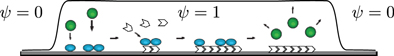
Figure 1. Schematic representation of the dynamics in the cell interior. The cellular domain is given by the region in which the phase field  . In this region, inactive NPFs, depicted in green, can become activated (blue). For the concreteness, we represent active NPFs as being bound to the substrate and inactive NPFs to be unbound. Active NPFs generate new filamentous actin, which in turn inactivates the NPFs.
Download figure:
Standard image High-resolution imageSince in equations (6) and (7) the diffusion terms are not directly coupled to the field ψ, NPFs can be transported outside the cell. For this reason, in our numerical integration scheme, NPFs having leaked out of the cell domain are removed in every time step by setting  and
and  , where we choose
  . Since the total number of NPFs is a conserved quantity, we also add a term to the NPF densities compensating for their loss outside the cell,
  and
and  . Here,
  and
and  are the respective amounts of degraded active and inactive NPFs outside the cell domain. We checked different ways for compensating for 'escaped' NPFs. The systems generated the states we report below practically independently of the method used. Similarly, the actin density T and orientation p can leak out of the cell domain. However, we will choose D = 0 in our simulations. As a consequence, this effect does not alter the solutions qualitatively and so we do not remove these fields explicitly.
2.4. Force balance
The cytoskeleton can only generate force dipoles such that the total momentum flux through the plasma membrane of a cell must vanish, if external forces are absent. In the overdamped regime considered here, this amounts to the sum of all internal forces acting on the cytoskeleton being zero. In the case considered here, the cytoskeleton can exchange momentum with the environment through interactions with the membrane and with the substrate it moves on. In addition, there might be a friction force originating from interactions between the surrounding fluid and the cell, but this force is negligibly small. While in our description forces do not appear explicitly, we can still interpret our dynamic equations in this respect. To this end we assume that the cytoskeleton adheres tightly to the substrate and neglect any actin flux relative to the substrate.
Let us consider force balance in a situation close to a sharp interface limit, that is,  is very small. At the membrane, three forces need to be considered. First of all, surface tension
  leads to a force density
  along the membrane. Here,
  , with χ being the membrane curvature and
  denoting the outward normal
  , see [27]. Dissipative (friction) forces are captured by
  , where
  is the (local) membrane velocity and ξ is the effective friction coefficient. Finally, there is the force
  exerted by the cytoskeleton on the membrane. This is given by
  . We will see below in the numerical solutions that actin is only pushing on the membrane, that is, p is pointing outwards. This is in contrast to systems containing molecular motors generating contractile stresses in the cytoskeleton [28, 41]. Locally, we arrive at the following kinematic condition for the membrane

We now return to our discussion of the global force balance. As stated above, the sum over all external forces acting on the cytoskeleton must vanish. Under the assumptions made above, we only consider the traction and membrane forces on actin. Explicitly, we have

where the integral is along the membrane and  . Let us emphasize that the traction forces are confined to the position of the membrane. This is because we do not consider any active stresses generated by the interaction of molecular motors with the actin network [31]. Indeed, the slime mold D. discoideum does not form focal adhesions and traction forces are essentially restricted to the outer boundaries [42].
3. Migration patterns generated by spontaneous polymerization waves
We investigate equations (1)–(7) by numerical integration in two dimensions on a square domain with periodic boundary conditions. Simulations start with a phase field  in a square of area
  and
and  elsewhere. The initial density of the NPFs is homogenous with a random perturbation of 30% within the region of
  . We solved equations (1)–(7) by a pseudo-spectral method.
As long as the polymerization velocity  or the detachment rate
  of the NPFs are small enough, the system will settle into a circular symmetric stationary state. In this case, the NPF densities decay monotonically from the cell center. The same is true for the actin density and the magnitude of the polarization. The polarization vector is pointing radially outwards corresponding to a topological point defect of charge +1 in the cell center. In this state there is a constant nucleator flux from the cell center to the cell periphery. Some features of the steady states are also present in the dynamic states we are going to discuss in the following. Firstly, the actin distribution is essentially the same as the nucleator distribution, see appendix
In the following, we show that by changing the polymerization velocity  and/or the nucleator deactivation rate
  , the system can self-organize into moving states. We will first discuss persistently moving (gliding) states and then consider a solution reminiscent of amoeboidal motion. Finally, we present cuts through the phase diagram of the system.
3.1. Directional motion
For large enough values of  and
and  , the system can spontaneously break the circular symmetry of the stationary state and evolve into a state of persistent motion, see figure 2 and supplementary movie S01, available at stacks.iop.org/njp/16/055007/mmedia. In such a state, the active NPFs localize at the leading edge and, hence, also the filament density T. The polarization field has topological defects at the maximum actin densities, see figure 3 and appendix
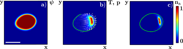
Figure 2. Snapshot of a directionally moving (gliding) state solution to equations (1)–(7). (a) Phase field ψ, (b) total actin density T and polarization p (white arrows), and (c) density of active NPFs  . In (b) and (c), the green line indicates the loci of
  . Parameter values are given in table B1 with
  , and
, and  . The scale bar is 0.19 λ.
Download figure:
Standard image High-resolution image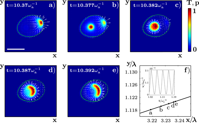
Figure 3. Actin dynamics in the gliding state. (a)–(e) Subsequent snapshots of the actin density T and the polarization p. (f) Corresponding trajectory of the phase field's center of mass. Letters indicate its position at the times corresponding to panels (a)–(e). Inset: absolute value of the cell velocity as a function of time. Parameters are as in figure 2. The scale bar is 0.19 λ.
Download figure:
Standard image High-resolution imageThese periodic changes in the distributions lead to oscillatory variations in the propulsion force, see figure 3(f), inset. As a result, the speed of the cell exhibits profound periodic oscillations similar to that observed in D. discoideum [44]. Periodic changes of the migration speed have also been observed in neutrophils [45], but there might be a consequence of  oscillations. The average propulsion velocity is largely independent of the polymerization velocity
  . Instead, it depends sensitively on the rates of actin nucleation and of nucleator binding and unbinding. This behavior can be rationalized by considering a dimensionless form of equations (1)–(7). As we show in appendix
  of active nucleators. This property also suggests that details of the actin polymerization process are not important for the overall system behavior. Indeed, other polymerization dynamics in combination with the NPF dynamics similar to the one used here have been found to spontaneously produce waves [14, 16, 18, 19]. Even though the polymerization velocity does not have a major impact on the wave's propagation velocity or the cell's migration speed, which are set by the rates of nucleator activation and inactivation as well as the actin nucleation rate, changes in
  can lead to the qualitative changes in the type of motion, as we will discuss now.
3.2. Irregular motion
Decreasing the growth velocity from  to
to  , the state changes qualitatively: the fragment is still moving, however, its trajectory is no longer straight; see figure 4(a). Instead it consists of curved segments that are interspersed by points at which the cell discontinuously changes direction. We would like to emphasize that this apparently random motion results from deterministic dynamic equations (1)–(7) without addition of noise.
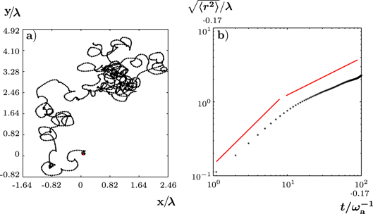
Figure 4. Irregularly moving solution of equations (1)–(7). (a) Trajectory of the center of mass of ψ over a time interval of 300  . (b) Root mean squared displacement for the trajectory shown in (a). Red lines indicate slopes 1 and 1/2. The value of the assembly velocity is
  . All other parameter values are as in figure 2.
Download figure:
Standard image High-resolution imageWe can characterize the trajectory by calculating its root mean squared displacement (RMSD)  ; see figure 4(b). On a short time scale
  , the RMSD grows essentially linearly with time. Then there is a cross-over to a region where the RMSD grows with an exponent close to but a little less than 1/2. The deviations from 1/2 might be due to finite size effects. We conclude that, within the accuracy of our calculations, the migration is diffusive in this state and can be described as a random walk. This conclusion is further supported by the velocity autocorrelation function, which decays rapidly. Furthermore, the curved segments have an equal probability of being curved in one or the other direction, making the random walk unbiased.
To obtain a better understanding of the processes underlying the formation of an irregularly moving state, let us consider the actin distribution T during an event of a discontinuous change in the direction of motion, see figure 5 and supplementary movie S02. Again the actin field is concentrated in a fraction of the cell domain. In contrast to actin 'blobs' in the gliding states, it now lacks a lateral symmetry axis, though. Instead it spirals along the cell membrane leading to curved segments of the trajectory (figure 5). Similar to the gliding states, in the irregularly moving state, too, the blobs have only a finite life-time. New blobs are then generated in the cell interior, which again leads to spiral motion. We could not detect any correlation between the orientations of two subsequent spirals. Consequently, the trajectory can change discontinuously. An additional feature of the dynamics is that a blob can break up into two or more parts, see figures 5(b), (c). This typically leads to changes in the curvature radius of the trajectories' curved segments.
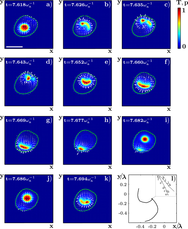
Figure 5. Details of a directional change of the trajectory presented in figure 4. (a)–(k) Snapshots of the actin density T and the polarization p. (l) The corresponding points of the center-of-mass trajectory. Inset: zoom into a part of the trajectory. Letters indicate its position at the times corresponding to panels (a)–(k). The scale bar is 0.19 λ.
Download figure:
Standard image High-resolution imageThe actin blobs develop into spirals if the cell size  is chosen to be sufficiently large, see below. We conclude that the irregular state essentially results from the intrinsic non-trivial spiral dynamics. Such dynamics is known from excitable systems with delayed inhibitor production [46] or more than two components [47], as well as from oscillatory media [33, 48].
3.3. Phase diagram
To obtain a more systematic understanding of the emerging states, we construct the phase diagram as a function of two most crucial parameters: the nucleator detachment rate  and the actin polymerization velocity
  , see figure 6. Before describing the phase diagram let us comment on the dependence of the system on the nucleation rate α and the nucleator activation rate
  . As the actin density follows the dynamics of the active nucleators closely, changing the value of α has a similar effect as changing the value of
  . Indeed, in the dynamic equations (1)–(7) only the product
  appears and
  . In contrast, increasing the value of
  has a similar effect as decreasing the value of
  .
.
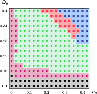
Figure 6. Phase diagram for equations (1) and (4)–(7) in terms of the actin dynamics as a function of the dimensionless nucleator detachment rate  and the dimensionless actin polymerization velocity
  . Dots: axially symmetric stationary states; squares: periodically appearing and vanishing blobs with (blue) and without (red) axial symmetry; triangles: stable (magenta) and unstable (green) spiral dynamics. Other parameters as in figure 2.
Download figure:
Standard image High-resolution imageWe classify the states in terms of the actin dynamics inside the cell. As noted in the previous sections, the actin distribution can be stationary and axially symmetric, see figure 7(a), it can organize into spirals, or form blobs of high concentration having a finite lifetime. The spiral states can be further divided into stable and unstable spirals, meaning that they incessantly break up, disappear, and nucleate again. Two examples of the former are shown in figures 7(b), (c); see also supplementary movies S04 and S05. The blobs can either be axially symmetric as discussed above for the gliding state or not. In the non-symmetric case, they move along the cell boundary, see figures 7(d)–(f) and supplementary movie S03. The appearance and disappearance of blobs is periodic in time not only for the axially symmetric blobs as we had seen above, but apparently also in the general case. From our numerical solutions it is not clear if the transition from spirals to blobs moving along the membrane is a bifurcation or a continuous transition. Let us also note that we did not detect regions of co-existence between the different states.

Figure 7. Actin distribution and polarization of solutions to equations (1)–(7) for different values of  and
and  . (a) Axially symmetric state for
  and
and  . (b) Stable rotating distribution for
  and
and  . (c) Stable spiral for
  and
and  . Large white arrows indicate the sense of rotation. (d)–(f) Subsequent snapshots of a non-symmetric blob for
  and
and  . Inset: corresponding trajectory of the cell's center of mass. Other parameters are as in figure 2. Scale bar: 0.19 λ.
Download figure:
Standard image High-resolution image
Different states of the internal actin dynamics correspond to different mobility patterns of the cell. In a stationary state, the cell's center of mass does obviously not move. In the case of stable spirals, the center of mass does not move either. The spiral arm moves along the membrane and induces a protrusion travelling along the membrane similar to observations made on spreading fibroblast [49, 50] and in drosophila cells with silenced Pak3, a homolog of p21-activated kinase [51]. Interestingly, Pak3 depleted cells show an increased actin-polymerization activity. In our case, however, protrusions are small and more work is needed to establish the relation between the polymerization waves in adhering cells and the ones studied here. Unstable spirals produce the irregular orbits presented above. Moving away from the spirals' stability threshold, the corresponding effective diffusion constant increases. For unstable blobs, the center of mass moves along trajectories reminiscent of Lissajous figures, see figure 7(f), inset. As the period necessary for circling along the cell perimeter approaches the lifetime of a blob, the trajectory approaches a circle. Finally, the axially symmetric blobs are associated with directional motion as discussed above.
The cell dynamics also depends on the typical cell volume  if all other parameters are fixed, such that the dynamics of the nucleator and actin fields spontaneously generate waves. Below a critical value, the cell remains immobile in a stationary state. Beyond this value, the cell moves directionally as in the phase indicated by the blue squares in figure 6. As the cell size is increased further, the system settles first into the randomly moving dynamic state. Alternatively, the system can assume the state with pinned center of mass and fluctuation of the cell boundary. For large cell volumes, the actin density formed a well-developed spiral, see supplementary movie S06.
In addition to the physical parameters discussed so far, the phase field parameters also have an impact on the states generated by the system. An obvious effect of increasing the diffusion constant  is a broadening of the interface, whereas the limit
  yields the sharp interface limit. In addition, larger values of
  also lead to a decreasing area of the cell: for the parameter values given in table B1, an increase of
  from 0.002 to 0.01, the area changed from 0.037
  to 0.03
  . Importantly, though, we could not detect a change in the state due to changes in
  .
.
This is different for changes in the value of β, which describes the coupling of the actin field to the interface and also depends on the actin polymerization rate. With increasing β we observe the same sequence of states as for increasing  and
and  : unstable spirals turn into periodically appearing and vanishing blobs, first without and then with axial symmetry. Finally, for decreasing values of , fluctuations in the cell area around the value
  increase. Below a critical value of , the circular symmetric shape of the cell is stable. In this case, the cell volume varies periodically corresponding to a breather state of the actin network.
4. Conclusions
In this work we used a phase-field model for the actin dynamics in cells to elucidate the impact of spontaneous polymerization waves on cell migration. In contrast to considering the dynamics of the cell boundary explicitly, the phase-field approach is numerically very efficient and better suited for parallel or GPU computing. We kept the phase-field dynamics simple and did not consider the effect of a finite bending rigidity, although this can be done as well [26, 27]. In this way we were able to scan large parts of the parameter space.
Similar to previous studies, we have found directionally moving states with the corresponding cell shape elongated in the direction of motion. This can be contrasted to systems that include actin contractility mediated by molecular motors, in which case cells are typically elongated in the direction perpendicular to the direction of motion [27, 28]. The cell shape can thus serve as an indicator of the relative importance of contractility versus polymerization during migration. In the directionally moving state, the actin dynamics oscillated within the reference system of the cell. This is different from a previous study on cell migration driven by spontaneous polymerization waves [43], where the actin distribution was stationary in the cell frame.
In addition to the directional migration, we found states of apparently random motion that are linked to spiral waves in the actin density and which had not been reported before. The ensuing cell movements are reminiscent of amoeboidal cell migration as it is displayed, for example, by human neutrophils. In particular, they show a rudimentary form of pseudopods, which have a comparatively short lifetime. This finding shows that amoeboidal motion might essentially result from the deterministic chaotic dynamics of the actin cytoskeleton, rather than as a consequence of thermal or molecular noise.
Our numerical solutions showed that the irregular motion is linked to the dynamics of spirals generated by the interplay of the NPFs and actin. Non-trivial spiral dynamics and spiral break-up is known from a number of excitable systems [46–48]. It will be interesting to apply the techniques developed in this context to further study the behavior of spiral actin waves. In this way, one could probably determine how the system parameters influence the key parameters of the irregular motion, notably, the corresponding effective diffusion constant. This parameter is important, for example, in the context of immune cells searching for infected cells as it influences the time needed to find a target cell. Immune cells thus might want to adapt their motion environmental conditions to increase their search efficiency [52].
Although we studied a specific mechanism of actin wave generation here, we might expect that the essential features we observed are largely independent of many details of this mechanism. Indeed, we observed that the speed at which the waves propagate is largely independent of the polymerization velocity  . This suggests that it should, for example, be irrelevant whether actin filaments treadmill or not. In this context it is noteworthy that the periodic variations in the propagation velocity, figure 3(f), inset, as well as the changes in propagation direction in the irregular state, figure 5, share essential features with observations on D. discoideum cells [44].
Many open questions remain. In particular, it would be interesting to study the influence of environmental cues on polymerization waves. Such a study could suggest possible mechanisms of signal transduction that are based on the intrinsic dynamics of the actin cytoskeleton. Most pressing at this stage, however, seem to be experimental studies that address the importance of polymerization waves for cell locomotion. Our calculations suggest that topological point defects in the actin network play an important role in this context. It remains a challenge to experimentally study their dynamics in crawling cells.
Acknowledgments
AD and KK thank the Materials Theory Institute of Argonne National Laboratory, and ISA and KK thank the Isaac Newton Institute, Cambridge, UK, where part of the work was accomplished, for the kind hospitality. The research of ISA was supported by the US DOE, Office of Basic Energy Sciences, Division of Materials Science and Engineering. The work of KK and AD was funded by the DFG through KR3430/1, the Graduate School 1276, and SFB 1027.
Appendix A.: Connection of dynamic equations (4) and (5) with a kinematic description of assembling actin filaments
Here, we show how (4) and (5) for the actin dynamics are related to the kinematic framework developed in [17]. There, filaments are assumed to be rigid rods of variable length  . The length increases with velocity
  due to polymerization at the barbed end and decreases with velocity
  because of depolymerization at the pointed end. The orientation of a filament is given by the unit vector
  pointing into the direction of its pointed end. In addition, filaments are degraded at rate
  and new filaments nucleate at rate
  , where
  is the local density of nucleation promoting as above.
The state of the system is described by the distribution function c of barbed ends, which depends on space and on filament orientation and length,  . Its time-evolution is given by

The spatial components of the current due to filament assembly are given by  , whereas its component in
  -space is
  . The diffusion term with the effective diffusion constant D accounts for fluctuations in the system. Finally, filament nucleation is captured by the boundary condition on the length current
  at
at  . Explicitly,
  .
.
We can integrate out the length dependence of c. Introducing the density  of pointed ends and the total actin density T at r of filaments with orientation
  , that is,
  and
and  , we obtain from equation (A.1)


Now, we expand the dependence of  and T on
  in terms of the moments in
  . Denoting
  ,
,  ,
,  , and
, and  , we obtain


where terms of order 2 and higher in  have been neglected.
Consider now the case  and
and  , where L is a typical length scale on which the density
  of pointed ends varies. Then,
  will essentially relax to zero and can be neglected. From equation (A.6), we then obtain
  . Hence, we finally arrive at

where  . Dropping the subscript 'tot' in equations (A.8) and (A.5) we obtain


Coupling these fields to the phase field ψ as indicated above, we arrive at equations (4) and (5).
Some comments on the relation of the present model with respect to previous works are in order. The dynamic equations (6) and (7) for the NPFs are the same as in [17, 43] except that no coupling to a phase field was present. The original equation (A.1) for the filaments accounts for the same processes as in the works cited, but in [17] the filament density referred to filament centers instead of plus-ends. Further analysis differed in these works as a moment expansion of the length dependence was considered in [17] and the angular dependence was kept in [43]. These differences do not qualitatively affect the actin dynamics, though.
Appendix B.: Parameters
For the numerical solution of equations (1)–(7), we provide here a dimensionless form along with the values of the dimensionless parameters used in this work.
To obtain a dimensionless form of equations (1)–(7), we scale time by the nucleator activation rate  and space by the diffusion length of inactive nucleators λ with
  . We then arrive at:


In these equations, the tilde indicates that quantities have been non-dimensionalized. Explicitly, we have  ,
,  ,
,  ,
,  ,
,  ,
,  ,
,  ,
,  ,
,  ,
,  ,
,  ,
, 
 ,
,  .
.
The parameters we have used throughout the work, unless stated otherwise, are listed in table B1. From these values, we deduce that the terms involving  and
and  dominate the dynamics in equations (B.2) and (B.3), which leaves us with
  and
and  . Considering the term of next higher order for the polarization p, we find that the gradients in T are the sources of the polarization explaining the existence of topological defects at the maxima of active nucleator density observed in the numerical solutions.
Table B1. The dimensionless parameter values used in the numerical solution.
| Value | Description | |
|---|---|---|

|
0.0 | Effective diffusion constant of actin filaments |

|
0.045 | Effective diffusion constant of active NPFs |

|
0.003 | Diffusion constant of the interface |

|
0.006 | Value of cooperativity |

|
0–0.4 | Deactivation rate of NPF |

|
0–0.4 | Polymerization velocity |

|
175.0 | Degradation rate |

|
120.0 | Initial density of inactive NPFs |

|
0.015 | Initial area of the interface |
|
|
4.0 | Stiffness of the constraint |

|
588.0 | Measure for the nucleation rate |

|
0.036 | Strength of the coupling |

|
118.0 | Sets the time scale for the interface |
Movie 1. (1.62 MB, MPG) Actin dynamics in the gliding state corresponding to figure 3.
Movie 2. (2.78 MB, MPG) Irregular state with spiral instability corresponding to figure 5.
Movie 3. (1.79 MB, MPG) Non-symmetric blob formation corresponding to figure 7(d)–(f).
Movie 4. (1.41 MB, MPG) Stable rotating solution corresponding to figure 7(b).
Movie 5. (1.40 MB, MPG) Stable one-armed spiral solution corresponding to figure 7(c).
Movie 6. (1.63 MB, MPG) Well-developed spiral solution for large cell volumes.