Quantum Fisher information as a signature of the superradiant quantum phase transition

Quantum phase transitions in many-body systems are of fundamental interest [1] and have potential applications in quantum information [2–7] and quantum metrology [8–15]. Consider, for instance, a collection of N two-level atoms interacting with a single-mode bosonic field, described by the Dicke model (with $\hbar =1$) [16]:

$$\begin{eqnarray}&&\hat{H}=\omega {{\hat{b}}^{\dagger }}\hat{b}+{{\omega }_{0}}{{\hat{J}}_{z}}+\frac{\lambda }{\sqrt{N}}({{\hat{b}}^{\dagger }}+\hat{b})({{\hat{J}}_{+}}+{{\hat{J}}_{-}}),\end{eqnarray} \tag{ 1 }$$

where $\hat{b}$ and ${{\hat{b}}^{\dagger }}$ are annihilation and creation operators of the bosonic field with oscillation frequency ω, which is nearly resonant with the atomic energy splitting ${{\omega }_{0}}$. The collective spin operators ${{\hat{J}}_{\pm }}\equiv {{\hat{J}}_{x}}\pm i{{\hat{J}}_{y}}={{\sum }_{k}}\hat{\sigma }_{k}^{\pm }$ and ${{\hat{J}}_{z}}={{\sum }_{k}}\hat{\sigma }_{k}^{z}/2$ obey the SU(2) Lie algebra, where $\hat{\sigma }_{k}^{\pm }$ and $\hat{\sigma }_{k}^{z}$ are Pauli operators of the kth atom. The atom-field coupling strength $\lambda \propto \sqrt{N/V}$ depends on the atomic density $N/V$. For a finite number of atoms N ($=2j$), the Hamiltonian (1) commutes with the parity operator $\hat{\Pi }={\rm exp} [i\pi ({{\hat{b}}^{\dagger }}\hat{b}+{{\hat{J}}_{z}}+j)]$, due to ${{\hat{\Pi }}^{\dagger }}{{\hat{J}}_{x}}\hat{\Pi }=-{{\hat{J}}_{x}}$ and ${{\hat{\Pi }}^{\dagger }}\hat{b}\hat{\Pi }=-\hat{b}$ [17]. As a result, the ground state of the finite-N Dicke model $\mid g\rangle$ does not exhibit any singularity or degeneracy. This can be understood by expanding the ground state in the basis $\{\mid n\rangle \otimes \mid \;j,m\rangle \}$, where $\mid n\rangle$ and $\mid \;j,m\rangle$ denote the Fock states of the field mode and the Dicke states of the atoms [18], respectively. For vanishing atom-field coupling strength λ, the ground state $\mid g\rangle =\mid 0\rangle \otimes \mid \;j,-j\rangle$ has a positive parity $\langle \hat{\Pi }\rangle =+1$; similarly for $\lambda >0$, due to the conserved parity, the ground state $\mid g\rangle$ consists of states with even number $n+m+j$, which results in vanishing coherence (i.e., $\langle {{\hat{J}}_{x}}\rangle =\langle \hat{b}\rangle =0$). However, in the thermodynamic limit (for finite $N/V$, as N and $V\to \infty$), the parity symmetry is spontaneously broken and the ground states with parities $\pm 1$ become degenerate in the superradiant phase (i.e., the symmetry-broken phase at $\lambda \geqslant {{\lambda }_{{\mbox{cr}}}}=\sqrt{{{\omega }_{0}}\omega }/2$) [19–31], leading to the bifurcation of both $\langle {{\hat{J}}_{x}}\rangle$ and $\langle \hat{b}\rangle$ [17].

Unlike the traditional phase transition of the Dicke model at a finite temperature [32], the superradiant quantum phase transition is driven by quantum fluctuations in the large-N limit. It is natural to ask in what different ways one can characterize such a quantum critical phenomenon in a realistic system. Several quantities, with various degrees of experimental accessibility, have been shown to be sensitive to the quantum criticality, such as the von Neumann entropy [7], the fidelity [33], and more recently the quantum squeezing of the field mode [34].

In this paper, we investigate the quantum Fisher information (QFI) of both the field state ${{\hat{\rho }}_{B}}={\mbox{T}}{{{\mbox{r}}}_{A}}(\mid g\rangle \langle g\mid )$ and the atomic state ${{\hat{\rho }}_{A}}={\mbox{T}}{{{\mbox{r}}}_{B}}(\mid g\rangle \langle g\mid )$, where ${\mbox{T}}{{{\mbox{r}}}_{A}}$ (${\mbox{T}}{{{\mbox{r}}}_{B}}$) is the partial trace of the ground state $\mid g\rangle$ over the atomic (bosonic field) degrees of freedom. The QFI is one of the central quantities used to qualify the utility of an input state [35, 36], especially in Mach–Zehnder (or, equivalently, Ramsey) interferometer-based phase or parameter estimation. The achievable phase sensitivity is well known to be limited by the quantum Cramér–Rao bound $\delta {{\varphi }_{{\rm min} }}\propto 1/\sqrt{F({{{\hat{\rho }}}_{{\mbox{in}}}},\hat{G})}$, where the QFI $F({{\hat{\rho }}_{{\mbox{in}}}},\hat{G})$ depends on the input state ${{\hat{\rho }}_{{\mbox{in}}}}$ and the choice of phase-shift generator $\hat{G}$ [36–38]. For a spin state ${{\hat{\rho }}_{{\mbox{in}}}}$ with fixed and finite N, the inequality $F({{\hat{\rho }}_{{\mbox{in}}}},\hat{G})>N$ provides not only a criterion of phase sensitivity better than the classical limit (i.e., $\delta {{\varphi }_{{\rm min} }}<1/\sqrt{N}$), but also a sufficient condition for the multiparticle entanglement of ${{\hat{\rho }}_{{\mbox{in}}}}$ [37].

Recently, Ma and Wang [12] have shown that the QFI is a sensitive probe of a quantum phase transition in the Lipkin–Meskhov–Glick model. Inspired by their work, we investigate the QFI of both the atomic state ${{\hat{\rho }}_{A}}$ and the field state ${{\hat{\rho }}_{B}}$ in the Dicke model. Unlike the finite-N spin systems studied elsewhere, the states we consider here are in general mixed states and the calculation of the QFI becomes more complex. Our numerical results show that near the critical point ${{\lambda }_{{\mbox{cr}}}}$, the QFI of each subsystem can surpass the classical limit due to the appearance of quadrature squeezing in ${{\hat{\rho }}_{A,B}}$. As the coupling strength $\lambda \gg {{\lambda }_{{\mbox{cr}}}}$, both ${{\hat{\rho }}_{A}}$ and ${{\hat{\rho }}_{B}}$ become highly mixed states, which leads to the QFI of the field returning to the classical limit, while for the atoms the QFI tends to zero. In the thermodynamic limit, we find that there exists analytical relationships between the QFI and the reduced variances, which show clearly the squeezing-induced enhancement of the QFI. More interestingly, we find that the derivative of $F({{\hat{\rho }}_{A,B}},\hat{G})$ for each subsystem is divergent at $\lambda ={{\lambda }_{{\mbox{cr}}}}$, similar to the fidelity of the ground state $\mid g\rangle$ in the one dimensional Ising chain [33]. This finding suggests that the QFI of the two subsystems in the Dicke model can identify the superradiant quantum phase transition.

Our paper is organized as follows. In section 2, we present numerical results of the QFI of the atomic and the field subsystems by exactly diagonalizing the finite-N Dicke Hamiltonian [21, 25]. In section 3, analytical results of the QFI and its relationship with the reduced variance for each subsystem are derived in the thermodynamic limit. Finally, we present a brief conclusion and discuss the role of the so-called ${{\hat{A}}^{2}}$ term.

We first examine the field state ${{\hat{\rho }}_{B}}={\mbox{T}}{{{\mbox{r}}}_{A}}(\mid g\rangle \langle g\mid )$ of the finite-N Dicke model by numerically evaluating the QFI with respect to ${{\hat{\rho }}_{B}}(\varphi )={\rm exp} (-i\varphi \hat{G}){{\hat{\rho }}_{B}}{\rm exp} (i\varphi \hat{G})$, where φ is an unknown phase shift and $\hat{G}$ is the phase-shift generator ($={{\hat{b}}^{\dagger }}\hat{b}$ for the single-mode field [38]). In general, the field state ${{\hat{\rho }}_{B}}(\varphi )$ is a mixed state and the QFI is given by [36–41]

$$\begin{eqnarray}&&F({{\hat{\rho }}_{B}},\hat{G})=4\mathop{\sum }\limits_{n}{{p}_{n}}\left( \Delta \hat{G} \right)_{n}^{2}-\mathop{\sum }\limits_{m\ne n}\frac{8{{p}_{m}}{{p}_{n}}}{{{p}_{m}}+{{p}_{n}}}\mid \langle {{\psi }_{m}}\mid \hat{G}\mid {{\psi }_{n}}\rangle {{\mid }^{2}},\end{eqnarray} \tag{ 2 }$$

where the weights $\{{{p}_{n}}\}$ are nonzero eigenvalues of ${{\hat{\rho }}_{B}}$, and $\{\mid {{\psi }_{n}}\rangle \}$ are the corresponding eigenvectors. The first term of equation (2) is a weighted average over the QFI for each pure state $\mid {{\psi }_{n}}\rangle$, and the variance is $(\Delta \hat{G})_{n}^{2}\equiv \langle {{\psi }_{n}}\mid {{\hat{G}}^{2}}\mid {{\psi }_{n}}\rangle -\mid \langle {{\psi }_{n}}\mid \hat{G}\mid {{\psi }_{n}}\rangle {{\mid }^{2}}$. The second term is simply a negative correction (cf [41]). For a pure coherent state $\mid \alpha \rangle$, with mean number of bosons $\bar{n}=\mid \alpha {{\mid }^{2}}$, the QFI of the bosonic field $F({{\hat{\rho }}_{B}},\hat{G})$, denoted shortly by ${{F}_{B}}$, is simply given by ${{F}_{B}}=4{{(\Delta {{\hat{b}}^{\dagger }}\hat{b})}^{2}}=4\bar{n}$. Therefore, the ultimate sensitivity is limited by $\delta \varphi _{{\rm min} }^{{\mbox{cl}}}=1/(2\sqrt{{\bar{n}}})$, known as the classical (or shot-noise) limit. A sub shot-noise-limited phase sensitivity with $\delta \varphi <\delta \varphi _{{\rm min} }^{{\mbox{cl}}}$ is achievable provided that ${{F}_{B}}>4\bar{n}$ (see figure 1(a)), which has also been shown to be a nonclassical criterion of ${{\hat{\rho }}_{B}}$ for the single-mode linear interferometer [42].

Zoom In Zoom Out Reset image size

The atoms in the ground state ${{\hat{\rho }}_{A}}={\mbox{T}}{{{\mbox{r}}}_{B}}(\mid g\rangle \langle g\mid )$ can also be used as a probe of a Ramsey interferometer. First, an external $\pi /2$-pulse is required to rotate the atomic spin about the ${{\hat{J}}_{y}}$ axis. Next, a phase shift $\varphi ={{\omega }_{0}}\tau$ is accumulated during free evolution under the Hamiltonian ${{\omega }_{0}}{{\hat{J}}_{z}}$. Finally, a second $\pi /2$-pulse is applied to extract the phase information. The total action of the pulses and the phase accumulation is equivalent with an unitary operator ${\rm exp} (-i\varphi {{\hat{J}}_{x}})$. Again, the QFI of the reduced atomic state ${{\hat{\rho }}_{A}}(\varphi )={\rm exp} (-i\varphi {{\hat{J}}_{x}}){{\hat{\rho }}_{A}}{\rm exp} (i\varphi {{\hat{J}}_{x}})$ is given by equation (2), where the phase-shift generator $\hat{G}$ is replaced by ${{\hat{J}}_{x}}$ and $\{\mid {{\psi }_{n}}\rangle \}$ are eigenvectors of ${{\hat{\rho }}_{A}}$ with nonzero weights ${{p}_{n}}$. For a coherent spin state $\mid \;j,-j\rangle =\mid \downarrow {{\rangle }^{\otimes N}}$, the QFI of the atoms is given by $F({{\hat{\rho }}_{A}},{{\hat{J}}_{x}})=4{{(\Delta {{\hat{J}}_{x}})}^{2}}=N$, so the sensitivity is limited by $\delta \varphi _{{\rm min} }^{{\mbox{cl}}}=1/\sqrt{N}$ (i.e., the classical limit). Hereafter, we denote the QFI of the atoms as ${{F}_{A}}$, to distinguish it from that of the bosonic field ${{F}_{B}}$.

In figure 1, we plot the scaled QFI of the field ${{F}_{B}}/(4\bar{n})$ and that of the atoms ${{F}_{A}}/N$ against the atom-field coupling strength λ. We first calculate the ground state for the finite-N system, which takes the form of [21, 25]:

$$\begin{eqnarray}&&\mid g\rangle =\mathop{\sum }\limits_{n=0}^{{{n}_{{\rm max} }}}\mathop{\sum }\limits_{m=-j}^{+j}{{c}_{n,m}}\mid n\rangle \otimes \mid \;j,m\rangle ,\end{eqnarray} \tag{ 3 }$$

where ${{n}_{{\rm max} }}$ is a cutoff photon number, $m\in [-j,+j]$ for $j=N/2$, and the probability amplitudes ${{c}_{n,m}}$ are obtained numerically by diagonalizing the Dicke Hamiltonian (1). Due to the conserved parity $\hat{\Pi }$, the Hilbert space only contains the states $\mid n\rangle \otimes \mid \;j,m\rangle$ with even excitation number $n+m+j$, which in turn gives the dimension of the subspace $[(N+1)({{n}_{{\rm max} }}+1)+1]/2$. In our numerical calculations, the value of ${{n}_{{\rm max} }}$ is increased until the quantities of interests remain unchanged [43]. Since the subspace is still huge, we evaluate the ground state for the number of atoms up to N = 20, limited by our computational resources. Next, for each subsystem ${{\hat{\rho }}_{A,B}}$, we can obtain the variances of the quadrature operators and the phase-shift generators. To solve the QFI, we further calculate the eigenvalues and the associated eigenvectors of ${{\hat{\rho }}_{A,B}}$ and insert them into equation (2). As depicted by the solid curves of figure 1(a), one can find that for vanishing λ, the QFI of the field ${{F}_{B}}/(4\bar{n})=0$ because the bosonic field is in a vacuum state, i.e., ${{\hat{\rho }}_{B}}=\mid 0\rangle \langle 0\mid$ at $\lambda =0$. In contrast, the QFI of the atoms is given by ${{F}_{A}}=N$ for the coherent spin state ${{\hat{\rho }}_{A}}=\mid \;j,-j\rangle \langle j,-j\mid$, as mentioned above. When the coupling λ increases up to its critical point ${{\lambda }_{{\mbox{cr}}}}$, the ground state contains a large number of excitations [21, 28] and ${{F}_{B}}$ begins to increase. It surpasses the classical limit around ${{\lambda }_{{\mbox{cr}}}}$ as the ratio ${{F}_{B}}/(4\bar{n})>1$ (see the solid lines of figure 1(a)). From figure 1(b), one can note that the QFI of ${{\hat{\rho }}_{A}}$ with small N cannot beat the classical limit; the ratio ${{F}_{A}}/N$ is always smaller than 1 and decreases monotonically with increasing λ. Only for a large enough number of atoms (say, $N>10$), can the scaled QFI ${{F}_{A}}/N$ be larger than 1 around the critical point ${{\lambda }_{{\mbox{cr}}}}$.

It is interesting to observe two key features of the finite-N Dicke model: (i) near the critical point ${{\lambda }_{{\mbox{cr}}}}$, both ${{\hat{\rho }}_{A}}$ and ${{\hat{\rho }}_{B}}$ provide enhanced QFI beyond the classical limits, although they are in general highly mixed states; (ii) for $\lambda \gg {{\lambda }_{{\mbox{cr}}}}$, the QFI of the field approaches the classical limit, i.e., ${{F}_{B}}\to 4\bar{n}$, while for the atoms, ${{F}_{A}}\to 0$. To understand this behavior we study in detail the quantum nature of ${{\hat{\rho }}_{A,B}}$ (see below). In section 3, we further present analytical results of the QFI in the thermodynamic limit (i.e., $N=\infty$), and find that both ${{F}_{B}}/(4\bar{n})$ and ${{F}_{A}}/N$ show critical behavior at $\lambda ={{\lambda }_{{\mbox{cr}}}}$.

The quantum nature of ${{\hat{\rho }}_{A,B}}$ can be partially visualized by the quasi-probability distribution of the atoms ${{Q}_{A}}(\theta ,\phi )=\langle \theta ,\phi \mid {{\hat{\rho }}_{A}}\mid \theta ,\phi \rangle$ and that of the bosonic field ${{Q}_{B}}(\alpha )=\langle \alpha \mid {{\hat{\rho }}_{B}}\mid \alpha \rangle$, where $\mid \alpha \rangle ={\rm exp} (\alpha {{\hat{b}}^{\dagger }}-{{\alpha }^{*}}\hat{b})\mid 0\rangle$ and $\mid \theta ,\phi \rangle ={\rm exp} (\eta {{\hat{J}}_{+}}-{{\eta }^{*}}{{\hat{J}}_{-}})\mid \;j,-j\rangle$ (with $\eta =\theta {{e}^{-i\phi }}/2$) denote coherent states of the two subsystems [18]. Overall, there is a one-to-one correspondence between ${{Q}_{A}}$ and ${{Q}_{B}}$, as depicted in figure 2. For vanishing λ, both ${{\hat{\rho }}_{A}}$ and ${{\hat{\rho }}_{B}}$ are also minimum-uncertainty states, which exhibit isotropic quasi-probability distributions ${{Q}_{A}}(\theta ,\phi )={{{\rm cos} }^{4j}}(\theta /2)$ and ${{Q}_{B}}(\alpha )={\rm exp} (-\mid \alpha {{\mid }^{2}})$ (see figure 2(a)). When λ crosses ${{\lambda }_{{\mbox{cr}}}}$, from figure 2(b), we find that both ${{Q}_{A}}$ and ${{Q}_{B}}$ become elliptical, implying the appearance of phase-squeezed states for the two subsystems.

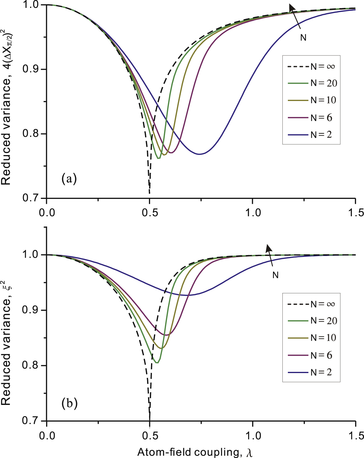
Zoom In Zoom Out Reset image size

To confirm the presence of nonclassical states at $\lambda \sim {{\lambda }_{{\mbox{cr}}}}$, we consider the quadrature squeezing of the field state ${{\hat{\rho }}_{B}}$, following the original calculations by Emary and Brandes [21]. As usual in quantum optics, we introduce a quadrature operator

$$\begin{eqnarray}&&{{\hat{X}}_{\sigma }}=\frac{1}{2}(\hat{b}{{e}^{-i\sigma }}+{{\hat{b}}^{\dagger }}{{e}^{i\sigma }}),\end{eqnarray} \tag{ 4 }$$

where the squeezing angle $\sigma \in [0,\pi /2]$ is to be determined. When $\sigma =0$ or $\pi /2$, the quadrature operator represents the amplitude or the phase component of the field mode, i.e., ${{\hat{X}}_{0}}=(\hat{b}+{{\hat{b}}^{\dagger }})/2$ or ${{\hat{X}}_{\pi /2}}=(\hat{b}-{{\hat{b}}^{\dagger }})/(2i)$. For vanishing coupling λ, the field is in the vacuum state $\mid 0\rangle$ and hence the variance ${{(\Delta {{\hat{X}}_{\sigma }})}^{2}}=1/4$, which is the classical limit of the field variance and is independent of the squeezing angle σ. This isotropic variance has been depicted in the right panel of figure 2(a). As the coupling λ increases, one finds

$$\begin{eqnarray*}&&{{(\Delta {{\hat{X}}_{\sigma }})}^{2}}=\frac{1}{4}+\frac{\operatorname{Re}\langle {{{\hat{b}}}^{2}}\rangle {\rm cos} (2\sigma )+\langle {{{\hat{b}}}^{\dagger }}\hat{b}\rangle }{2},\end{eqnarray*}$$

where we have used $\langle \hat{b}\rangle =0$ and $\langle {{\hat{b}}^{2}}\rangle \in \mathbb{R}$, due to the parity symmetry ${{\hat{\Pi }}^{\dagger }}\hat{b}\hat{\Pi }=-\hat{b}$ and the real atom-field coupling λ. Minimizing ${{(\Delta {{\hat{X}}_{\sigma }})}^{2}}$ with respect to σ, we obtain the optimal squeezing angle ${{\sigma }_{{\mbox{op}}}}=0$ or $\pi /2$. Our numerical result in figure 2(b) suggests ${{\sigma }_{{\mbox{op}}}}=\pi /2$, which means that the optimal squeezing occurs along the ${{\hat{X}}_{\pi /2}}$ axis with the reduced variance ${{(\Delta {{\hat{X}}_{\pi /2}})}^{2}}$ smaller than the classical limit $1/4$. In figure 3(a), we confirm that the degree of squeezing $4{{(\Delta {{\hat{X}}_{\pi /2}})}^{2}}<1$, and that it is minimized at $\lambda \sim {{\lambda }_{{\mbox{cr}}}}$ for large enough N.

Zoom In Zoom Out Reset image size

Similarly, one can consider the spin squeezing of the atomic state ${{\hat{\rho }}_{A}}$. Due to the conserved parity, the atoms have vanishing coherence $\langle {{\hat{J}}_{+}}\rangle =0$ and hence the total spin $\langle \hat{J}\rangle =(0,0,\langle {{\hat{J}}_{z}}\rangle )$, similar to that of the Lipkin–Meshkov–Glick model [4–6, 12]. To quantify the degree of spin squeezing [43–49], one can introduce a spin component ${{\hat{J}}_{\phi }}={{\hat{J}}_{x}}{\rm cos} \phi +{{\hat{J}}_{y}}{\rm sin} \phi$, which is normal to the total spin. Again, the squeezing angle ϕ is to be determined. Since $\langle {{\hat{J}}_{\phi }}\rangle =0$, we obtain the variance of ${{\hat{J}}_{\phi }}$ as

$$\begin{eqnarray*}&&{{\left( \Delta {{J}_{\phi }} \right)}^{2}}=\frac{1}{2}[\langle \hat{J}_{x}^{2}+\hat{J}_{y}^{2}\rangle +\operatorname{Re}\langle \hat{J}_{+}^{2}\rangle {\rm cos} (2\phi )],\end{eqnarray*}$$

where we have used Im $\langle \hat{J}_{+}^{2}\rangle \equiv \langle {{\hat{J}}_{x}}{{\hat{J}}_{y}}+{{\hat{J}}_{y}}{{\hat{J}}_{x}}\rangle =0$. It is easy to find the optimal squeezing angle ${{\phi }_{{\mbox{op}}}}=0$ or $\pi /2$ [45], and the left panel of figure 2(b) suggests ${{\phi }_{{\mbox{op}}}}=\pi /2$, corresponding to spin squeezing and anti-squeezing in the ${{\hat{J}}_{y}}$ and the ${{\hat{J}}_{x}}$ axes, respectively. A spin squeezed state is defined if the reduced variance of ${{\hat{J}}_{y}}$ is smaller than the classical limit $N/4$ [43–49]. As shown in figure 3(b), one can see that the squeezing parameter ${{\xi }^{2}}=4{{(\Delta {{\hat{J}}_{y}})}^{2}}/N$ is minimized around ${{\lambda }_{{\mbox{cr}}}}$.

From the solid lines of figure 1, we also note that as the coupling $\lambda \gg {{\lambda }_{{\mbox{cr}}}}$, the QFI of the field ${{F}_{B}}\to 4\bar{n}$, while for the atoms ${{F}_{A}}\to 0$. This behavior can be understood by examining the ground state of the finite-N Dicke Hamiltonian with $\lambda \to \infty$ [50–52]. In this ultra-strong coupling regime, the number of bosons $\bar{n}\propto {{\lambda }^{2}}\to \infty$ and hence the dominant term of the Dicke Hamiltonian is given by ${{\hat{H}}_{0}}=\omega {{\hat{b}}^{\dagger }}\hat{b}+2\lambda (\hat{b}+{{\hat{b}}^{\dagger }}){{\hat{J}}_{x}}/\sqrt{N}$. Minimizing the energy of ${{\hat{H}}_{0}}$ with respect to a product of coherent states $\mid \alpha \rangle \otimes \mid \;j,m{{\rangle }_{x}}$, one can obtain the atomic state ${{\hat{\rho }}_{A}}={{(\mid \;j,+j\rangle }_{xx}}{{\langle j,+j\mid +\mid \;j,-j\rangle }_{xx}}\langle j,-j\mid )/2$, where $\mid \;j,\pm j{{\rangle }_{x}}$, being eigenvectors of ${{\hat{J}}_{x}}$, provide the variances $(\Delta {{\hat{J}}_{x}})_{\pm }^{2}=0$. Therefore, from equation (2) we have ${{F}_{A}}\to 0$ as $\lambda \to \infty$. Similarly, the field state is given by ${{\hat{\rho }}_{B}}=(\mid +{{\alpha }_{0}}\rangle \langle +{{\alpha }_{0}}\mid +\mid -{{\alpha }_{0}}\rangle \langle -{{\alpha }_{0}}\mid )/2$, where $\mid \pm {{\alpha }_{0}}\rangle$, with the amplitude ${{\alpha }_{0}}=\lambda \sqrt{N}/\omega$, denoting coherent states [50–52]. It is easy to find that as the amplitude ${{\alpha }_{0}}$ ($\propto \lambda$) $\to \infty$, the two coherent states $\mid \pm {{\alpha }_{0}}\rangle$, almost orthogonal with each other, provide the variances $(\Delta {{\hat{b}}^{\dagger }}\hat{b})_{\pm }^{2}=\alpha _{0}^{2}=\bar{n}$. As a result, we obtain the total QFI of the bosonic field ${{F}_{B}}\approx 4{{\sum }_{\pm }}{{p}_{\pm }}(\Delta {{\hat{b}}^{\dagger }}\hat{b})_{\pm }^{2}=4\bar{n}$ (due to ${{p}_{\pm }}=1/2$), leading to the ratio ${{F}_{B}}/(4\bar{n})\to 1$ as $\lambda \to \infty$.

When the coupling $\lambda \gg {{\lambda }_{{\mbox{cr}}}}$, the quasi-probability distribution of ${{\hat{\rho }}_{A,B}}$ contains two contributions, i.e., ${{Q}_{A,B}}=({{I}_{-}}+{{I}_{+}})/2$, with ${{I}_{\pm }}={{[1\pm {\rm sin} (\theta ){\rm cos} (\phi )]}^{N}}/{{2}^{N}}$ for the atoms and ${{I}_{\pm }}={\rm exp} (-\mid \alpha \pm {{\alpha }_{0}}{{\mid }^{2}})$ for the bosonic field, as illustrated in figure 2(c). In addition, we obtain the reduced variances ${{(\Delta {{\hat{J}}_{y}})}^{2}}=N/4$ (i.e., ${{\xi }^{2}}=1$) and ${{(\Delta {{\hat{X}}_{\pi /2}})}^{2}}=1/4$ (see the solid curves in figure 3), as well as the increased variances ${{(\Delta {{\hat{X}}_{0}})}^{2}}=\alpha _{0}^{2}+1/4$ and ${{(\Delta {{\hat{J}}_{x}})}^{2}}={{N}^{2}}/4$, which have been confirmed by [53].

In this section, we first briefly review the quantum critical behavior of the Dicke model in the thermodynamic limit based on the solution outlined by Emary and Brandes [21], and then present analytical results of the QFI for the field and the atomic subsystems.

The standard procedure for the diagonalization of the Dicke Hamiltonian consists of four steps [21]. First, performing the Holstein–Primakoff transformation ${{\hat{J}}_{+}}={{({{\hat{J}}_{-}})}^{\dagger }}={{\hat{a}}^{\dagger }}\sqrt{N-{{{\hat{a}}}^{\dagger }}\hat{a}}$ and ${{\hat{J}}_{z}}={{\hat{a}}^{\dagger }}\hat{a}-N/2$, one can write down the Dicke Hamiltonian and the parity in terms of bosonic operators $\hat{a}$ and $\hat{b}$. Second, the operators $\hat{a}$ and $\hat{b}$ are decomposed as

$$\begin{eqnarray}&&\hat{a}=\delta \hat{a}\pm {{\alpha }_{s}},\quad \hat{b}=\delta \hat{b}\mp {{\beta }_{s}},\end{eqnarray} \tag{ 5 }$$

where ${{\alpha }_{s}}$ (${{\beta }_{s}}$) denotes the mean-field part and $\delta \hat{a}$ ($\delta \hat{b}$) the quantum fluctuation for each subsystem. Third, one obtains the Dicke Hamiltonian up to quadratic order in $\delta \hat{a}$ and $\delta \hat{b}$ by eliminating their linear terms, which gives the solution for the mean field parts [21]:

$$\begin{eqnarray}&&{{\alpha }_{s}}=\sqrt{\frac{N(1-\mu )}{2}},\quad {{\beta }_{s}}=\frac{\lambda }{\omega }\sqrt{N(1-{{\mu }^{2}})},\end{eqnarray} \tag{ 6 }$$

where the order parameters ${{\alpha }_{s}}$ and ${{\beta }_{s}}$ are vanishing for $\mu =1$ in the normal phase (i.e., $\lambda <{{\lambda }_{{\mbox{cr}}}}=\sqrt{\omega {{\omega }_{0}}}/2$), and ${{\alpha }_{s}}$, ${{\beta }_{s}}\sim O(\sqrt{N})$ for $\mu ={{({{\lambda }_{{\mbox{cr}}}}/\lambda )}^{2}}<1$ in the superradiant phase; the parameter μ allows a unified description in both phases ⁶ . Finally, one can diagonalize the effective Hamiltonian by introducing the Bogoliubov transformation: ${{\hat{q}}_{1}}={{\hat{X}}_{B}}{\rm cos} \gamma -{{\hat{X}}_{A}}{\rm sin} \gamma$ and ${{\hat{q}}_{2}}={{\hat{X}}_{B}}{\rm sin} \gamma +{{\hat{X}}_{A}}{\rm cos} \gamma$, where ${{\hat{q}}_{1,2}}$ denote the position operators of the polaritons and ${{\hat{X}}_{A,B}}$ are that of the atoms (A) and the bosonic field (B), i.e., ${{\hat{X}}_{A}}\propto (\delta {{\hat{a}}^{\dagger }}+\delta \hat{a})$ and ${{\hat{X}}_{B}}\propto (\delta {{\hat{b}}^{\dagger }}+\delta \hat{b})$. For the mixing angle γ given by ${\rm tan} (2\gamma )=4\lambda \sqrt{{{\omega }_{0}}\omega \mu }/[{{({{\omega }_{0}}/\mu )}^{2}}-{{\omega }^{2}}]$, one can obtain the Hamiltonian of the two-mode polaritons, with the excitation energies ${{\varepsilon }_{k}}$ (for k = 1, 2) determined by [21],

$$\begin{eqnarray}&&\varepsilon _{k}^{2}=\frac{{{\omega }^{2}}+{{\left( {{\omega }_{0}}/\mu \right)}^{2}}}{2}+\frac{{{(-1)}^{k}}}{2}\sqrt{{{\left[ {{\omega }^{2}}-{{\left( {{\omega }_{0}}/\mu \right)}^{2}} \right]}^{2}}+{{\left( 4\lambda \right)}^{2}}\omega {{\omega }_{0}}\mu },\end{eqnarray} \tag{ 7 }$$

where μ takes different values in the two phases (see footnote 6). In the position space of the polaritons, the ground-state wave function is given by ${{\Psi }_{g}}({{q}_{1}},{{q}_{2}})\equiv \langle {{q}_{1}},{{q}_{2}}\mid g\rangle {\mkern 1mu} ={\mkern 1mu} {{({{\varepsilon }_{1}}{{\varepsilon }_{2}}/{{\pi }^{2}})}^{1/4}}{\rm exp} [-({{\varepsilon }_{1}}q_{1}^{2}+{{\varepsilon }_{2}}q_{2}^{2})/2]$, which, according to the Bogoliubov transformation, can also be expressed in the coordinates of the atomic and the field operators ${{\hat{X}}_{A,B}}$.

The two possible shifts in equation (5) correspond to opposite spatial displacements of the ground state in position space, due to ${{\hat{X}}_{A}}=\sqrt{{{\omega }_{0}}/\tilde{\omega }}({{\hat{x}}_{A}}\mp {{\alpha }_{s}}\sqrt{2/{{\omega }_{0}}})$ and ${{\hat{X}}_{B}}={{\hat{x}}_{B}}\pm {{\beta }_{s}}\sqrt{2/\omega }$, where $\tilde{\omega }={{\omega }_{0}}(1+\mu )/2\mu$ (see footnote 6) and ${{\hat{x}}_{A,B}}$ are the position operators before the displacements. We first consider the atomic state ${{\hat{\rho }}_{A}}$ under one choice of the displacements. The reduced density matrix of the atoms can now be obtained by integrating ${{\Psi }_{g}}\Psi _{g}^{*}$ over the coordinate of the field operator ${{\hat{X}}_{B}}$, as done in [7]. The result has the same form as that of a thermal oscillator (see appendix, also [54]), with unit mass and the effective oscillation frequency

$$\begin{eqnarray}&&\Omega =\frac{{{\varepsilon }_{1}}{{\varepsilon }_{2}}}{{{\varepsilon }_{1}}{{c}^{2}}+{{\varepsilon }_{2}}{{s}^{2}}}\sqrt{1+\frac{{{\left( {{\varepsilon }_{1}}-{{\varepsilon }_{2}} \right)}^{2}}{{c}^{2}}{{s}^{2}}}{{{\varepsilon }_{1}}{{\varepsilon }_{2}}}},\end{eqnarray} \tag{ 8 }$$

where we have set $c={\rm cos} \gamma$, $s={\rm sin} \gamma$, and ${\rm cosh} (\beta \Omega )=1+2{{\varepsilon }_{1}}{{\varepsilon }_{2}}{{[{{({{\varepsilon }_{1}}-{{\varepsilon }_{2}})}^{2}}{{c}^{2}}{{s}^{2}}]}^{-1}}$, with $\beta ={{({{k}_{B}}T)}^{-1}}$ and the Boltzmann constant ${{k}_{B}}$. In the Fock basis of the thermal oscillator [54], the reduced density matrix of the atoms can be expressed as

$$\begin{eqnarray}&&{{\hat{\rho }}_{A}}=\frac{{{e}^{-\beta {{{\hat{H}}}_{A}}}}}{{\mbox{Tr}}{{e}^{-\beta {{{\hat{H}}}_{A}}}}}=\mathop{\sum }\limits_{n}{{p}_{n}}\mid {{\psi }_{n}}\rangle \langle {{\psi }_{n}}\mid ,\end{eqnarray} \tag{ 9 }$$

where ${{\hat{H}}_{A}}=(\hat{P}_{A}^{2}+{{\Omega }^{2}}\hat{X}_{A}^{2})/2$ is the effective Hamiltonian of the thermal oscillator [7], with the eigenvectors $\mid {{\psi }_{n}}\rangle \equiv {{(\hat{a}_{\Omega }^{\dagger })}^{n}}\mid 0\rangle /\sqrt{n!}$ and the eigenvalues ${{p}_{n}}\equiv \langle {{\psi }_{n}}\mid {{\hat{\rho }}_{A}}\mid {{\psi }_{n}}\rangle ={\rm exp} (-n\beta \Omega )$ $[1-{\rm exp} (-\beta \Omega )]$. Here, the momentum operator ${{\hat{P}}_{A}}$ can be expressed by the atomic fluctuation $\delta \hat{a}$, or the annihilation operator of the thermal oscillator ${{\hat{a}}_{\Omega }}$, i.e., ${{\hat{P}}_{A}}=i\sqrt{\tilde{\omega }/2}(\delta {{\hat{a}}^{\dagger }}-\delta \hat{a})=i\sqrt{\Omega /2}(\hat{a}_{\Omega }^{\dagger }-{{\hat{a}}_{\Omega }})$. The position operator of the atoms ${{\hat{X}}_{A}}$ is similarly defined, ${{\hat{X}}_{A}}=(\delta {{\hat{a}}^{\dagger }}+\delta \hat{a})/\sqrt{2\tilde{\omega }}=(\hat{a}_{\Omega }^{\dagger }+{{\hat{a}}_{\Omega }})/\sqrt{2\Omega }$.

As discussed in [21], the two displacements result in doubly degenerate and orthogonal ground states in the symmetry-broken (i.e., superradiant) phase, which in turn gives the different atomic states $\hat{\rho }_{A}^{\pm }$ corresponding to each possible displacement. We can also diagonalize each state in the two ortho-normalized Fock basis $\{\mid \psi _{n}^{\pm }\rangle \}$, with $\langle \psi _{n}^{\pm }\mid \psi _{{{n}^{^{\prime} }}}^{\pm }\rangle ={{\delta }_{n,{{n}^{^{\prime} }}}}$ and $\langle \psi _{n}^{\pm }\mid \psi _{{{n}^{^{\prime} }}}^{\mp }\rangle =0$. The total atomic state is often taken to be an incoherent superposition of both possible displacements $\hat{\rho }_{A}^{\pm }$ with the same weights, i.e., ${{\hat{\rho }}_{A}}=(\hat{\rho }_{A}^{+}+\hat{\rho }_{A}^{-})/2$. Note that the collective spin operators under the two displacements take the form

$$\begin{eqnarray}&&{{\hat{J}}_{x}}=\frac{N-2\alpha _{s}^{2}}{2\sqrt{N-\alpha _{s}^{2}}}(\delta {{\hat{a}}^{\dagger }}+\delta \hat{a})\pm {{\alpha }_{s}}\sqrt{N-\alpha _{s}^{2}}+O({{N}^{0}}),\end{eqnarray} \tag{ 10 }$$

$$\begin{eqnarray}&&{{\hat{J}}_{y}}=\frac{\sqrt{N-\alpha _{s}^{2}}}{2i}(\delta {{\hat{a}}^{\dagger }}-\delta \hat{a})+O({{N}^{0}}),\end{eqnarray} \tag{ 11 }$$

and ${{\hat{J}}_{z}}=(\delta {{\hat{a}}^{\dagger }}\pm {{\alpha }_{s}})(\delta \hat{a}\pm {{\alpha }_{s}})-N/2$, where the terms $\sim O({{N}^{0}})$ are negligible in the thermodynamic limit. Using the self-consistent condition $\langle \delta \hat{a}\rangle =0$ [21], it is easy to obtain the expectation values ${{\langle {{\hat{J}}_{x}}\rangle }_{\pm }}=\pm {{\alpha }_{s}}\sqrt{N-\alpha _{s}^{2}}$ and ${{\langle {{\hat{J}}_{y}}\rangle }_{\pm }}=0$ for each $\hat{\rho }_{A}^{\pm }$. A 50:50 weighted average over ${{\langle {{\hat{J}}_{x}}\rangle }_{\pm }}$ gives $\langle {{\hat{J}}_{x}}\rangle =\langle {{\hat{J}}_{y}}\rangle =0$ for the total density matrix ${{\hat{\rho }}_{A}}$. As in the previous finite-N case, the squeezing parameter is given by ${{\xi }^{2}}=4\langle \hat{J}_{y}^{2}\rangle /N$, with its explicit form

$$\begin{eqnarray}&&{{\xi }^{2}}=\frac{\mu \Omega }{{{\omega }_{0}}}\frac{{\rm exp} (\beta \Omega )+1}{{\rm exp} (\beta \Omega )-1}=\frac{\mu }{2{{\omega }_{0}}}\left( {{\varepsilon }_{1}}+{{\varepsilon }_{2}}+\frac{\omega _{0}^{2}/{{\mu }^{2}}-{{\omega }^{2}}}{{{\varepsilon }_{1}}+{{\varepsilon }_{2}}} \right),\end{eqnarray} \tag{ 12 }$$

where, in the the last step, we have dropped the intermediate quantities $\Omega$ and ${\rm exp} (\beta \Omega )$ (for details, please see the appendix). The reduced variance $\langle \hat{J}_{y}^{2}\rangle \propto \langle {{(\delta {{\hat{a}}^{\dagger }}-\delta \hat{a})}^{2}}\rangle$ can also be obtained from previous works [21]. To solve the QFI, one has to diagonalize the reduced density matrix as equation (9), and then calculate the QFI for each $\hat{\rho }_{A}^{\pm }$ using equation (2). Since both contributions from $\hat{\rho }_{A}^{\pm }$ are the same, we obtain the total QFI of the atoms (see appendix)

$$\begin{eqnarray}&&{{F}_{A}}=\frac{N\mu {{\omega }_{0}}}{\Omega }\frac{{\rm exp} (\beta \Omega )-1}{{\rm exp} (\beta \Omega )+1},\end{eqnarray} \tag{ 13 }$$

which has an exact relationship with the reduced variance, ${{F}_{A}}{{\xi }^{2}}=N{{\mu }^{2}}$ (see footnote 6). This finding can be used to verify that the enhanced QFI beyond the classical limit is induced by the squeezing. One can see this from equation (12). The squeezing parameter at the critical point is given by ${{\xi }^{2}}={{\omega }_{0}}{{({{\omega }^{2}}+\omega _{0}^{2})}^{-1/2}}<1$ due to ${{\varepsilon }_{1}}=0$ and ${{\varepsilon }_{2}}={{({{\omega }^{2}}+\omega _{0}^{2})}^{1/2}}$, which in turn leads to ${{F}_{A}}/N={{\xi }^{-2}}>1$ at $\lambda ={{\lambda }_{{\mbox{cr}}}}$.

For the field subsystem, one can also obtain the reduced density matrix $\hat{\rho }_{B}^{\pm }$ for each displacement, similar to equation (9), but with different oscillation frequency $\Omega {{\mid }_{c\leftrightarrow s}}$, i.e., interchanging c and s in equation (8). Again, we assume that the total field state is a mixture of $\hat{\rho }_{B}^{\pm }$, which can be diagonalized in the Fock basis $\{\mid \psi _{n}^{\pm }\rangle \}$. With the self-consistent condition $\langle \delta \hat{b}\rangle =0$, it is easy to obtain $\langle {{\hat{X}}_{\pi /2}}\rangle =\langle {{\hat{P}}_{B}}\rangle /\sqrt{2\omega }=0$ [21], where ${{\hat{P}}_{B}}=i\sqrt{\omega /2}$ $(\delta {{\hat{b}}^{\dagger }}-\delta \hat{b})=i\sqrt{\Omega /2}(\hat{b}_{\Omega }^{\dagger }-{{\hat{b}}_{\Omega }})$ and ${{\hat{X}}_{\pi /2}}$ is the quadrature operator of the bosonic field, defined by equation (4). For each $\hat{\rho }_{B}^{\pm }$, we find that the reduced variances $(\Delta {{\hat{X}}_{\pi /2}})_{\pm }^{2}={{\langle \hat{P}_{B}^{2}\rangle }_{\pm }}/(2\omega )$ take the same form (see appendix), and therefore

$$\begin{eqnarray}&&{{\left( \Delta {{{\hat{X}}}_{\pi /2}} \right)}^{2}}=\frac{\Omega }{4\omega }\frac{{\rm exp} (\beta \Omega )+1}{{\rm exp} (\beta \Omega )-1}=\frac{1}{8\omega }\left( {{\varepsilon }_{1}}+{{\varepsilon }_{2}}-\frac{\omega _{0}^{2}/{{\mu }^{2}}-{{\omega }^{2}}}{{{\varepsilon }_{1}}+{{\varepsilon }_{2}}} \right).\end{eqnarray} \tag{ 14 }$$

Again, we have removed the intermediate quantities $\Omega$ and ${\rm exp} (\beta \Omega )$ in the the last step. The QFI of the field mode depends on the matrix elements $\langle \psi _{m}^{\pm }\mid \hat{G}\mid \psi _{n}^{\pm }\rangle$, where $\hat{G}={{\hat{b}}^{\dagger }}\hat{b}=(\delta {{\hat{b}}^{\dagger }}\mp {{\beta }_{s}})(\delta \hat{b}\mp {{\beta }_{s}})$ denotes the phase-shift generator and $\delta {{\hat{b}}^{\dagger }}\pm \delta \hat{b}\;\propto$ $(\hat{b}_{\Omega }^{\dagger }\pm {{\hat{b}}_{\Omega }})$, as mentioned above. After some tedious calculations, we obtain the total QFI of the field mode (see appendix)

$$\begin{eqnarray}&&{{F}_{B}}=\frac{{{\left( {{\omega }^{2}}-{{\Omega }^{2}} \right)}^{2}}}{2{{\omega }^{2}}{{\Omega }^{2}}}\frac{{{\left[ {\rm exp} (\beta \Omega )+1 \right]}^{2}}}{{\rm exp} (2\beta \Omega )+1}+\frac{4\omega \beta _{s}^{2}}{\Omega }\frac{{\rm exp} (\beta \Omega )-1}{{\rm exp} (\beta \Omega )+1},\end{eqnarray} \tag{ 15 }$$

where ${{\beta }_{s}}$ is the order parameter, given by equation (6). In the normal phase, the first term of equation (15) dominates due to ${{\beta }_{s}}=0$. On the contrary, for the superradiant phase, the first term vanishes quickly and the second term becomes important due to the macroscopic occupation $\beta _{s}^{2}\sim O(N)\to \infty$, which gives a simple relation ${{F}_{B}}{{(\Delta {{\hat{X}}_{\pi /2}})}^{2}}\approx \beta _{s}^{2}\approx \bar{n}$ (see appendix for the explicit form of $\bar{n}$).

Our above results, equations (12)–(15), dependent upon the parameter μ, are valid for both phases (see footnote 6). In figures 1 and 3, we plot the scaled QFI and the reduced variances of ${{\hat{\rho }}_{A,B}}$ as a function of the atom-field coupling $\lambda$. For the vanishing coupling λ, we have ${{\xi }^{2}}={{F}_{A}}/N=4{{(\Delta {{\hat{X}}_{\pi /2}})}^{2}}=1$ and ${{F}_{B}}=0$ (as $\Omega =\omega$), due to $\mu =1$, ${{\alpha }_{s}}={{\beta }_{s}}=0$, and ${{\varepsilon }_{1}}+{{\varepsilon }_{2}}=\omega +{{\omega }_{0}}$. When the coupling increases up to ${{\lambda }_{{\mbox{cr}}}}$, the lower-branch polaritonic energy is gapless, i.e., ${{\varepsilon }_{1}}=0$ and ${{\varepsilon }_{2}}={{({{\omega }^{2}}+\omega _{0}^{2})}^{1/2}}$, so the reduced variance of the field $4{{(\Delta {{\hat{X}}_{\pi /2}})}^{2}}=\omega {{({{\omega }^{2}}+\omega _{0}^{2})}^{-1/2}}<1$ and hence ${{F}_{B}}/(4\bar{n})\approx 1/[4{{(\Delta {{\hat{X}}_{\pi /2}})}^{2}}]>1$, similar to that of the atomic subsystem. From the dashed lines of figures 1 and 3, one can easily see that at the critical point ${{\lambda }_{{\mbox{cr}}}}=1/2$ (on resonance with $\omega {{\omega }_{0}}=1$), the scaled QFI ${{F}_{A}}/N={{F}_{Q}}/(4\bar{n})\to \sqrt{2}$ due to ${{\xi }^{2}}=4{{(\Delta {{\hat{X}}_{\pi /2}})}^{2}}=1/\sqrt{2}$. As the coupling $\lambda \to \infty$, the excitation energies ${{\varepsilon }_{1}}\to \omega$ and ${{\varepsilon }_{2}}\to {{\omega }_{0}}/\mu$, yielding ${{\xi }^{2}}\to 1$ and ${{F}_{A}}/N\approx {{\mu }^{2}}\to 0$; while for the bosonic field, we have $\Omega \approx \omega$ and ${\rm exp} (\beta \Omega )\to \infty$, so ${{(\Delta {{\hat{X}}_{\pi /2}})}^{2}}\to 1/4$ and ${{F}_{B}}/(4\bar{n})\to 1$, returning to the classical limit.

Before closing, we study the critical behavior of the QFI of the atoms ${{F}_{A}}/N$ and that of the field mode ${{F}_{B}}/(4\bar{n})$ at $\lambda \sim {{\lambda }_{{\mbox{cr}}}}$. The critical exponents of a quantum phase transition are manifested in the behavior of the excitation energies [1]. For the Dicke model, it has been shown that the lower-branch excitation energy vanishes at $\lambda ={{\lambda }_{{\mbox{cr}}}}$ as ${{\varepsilon }_{1}}\sim \mid \lambda -{{\lambda }_{{\mbox{cr}}}}{{\mid }^{2\nu }}$, with the critical exponent $\nu =1/4$ [21]. Recently, Nataf et al [34] have found that a product of variances of the field mode $\Delta {{\hat{X}}_{0}}\Delta {{\hat{X}}_{\pi /2}}$ diverges as $\mid \lambda -{{\lambda }_{{\mbox{cr}}}}{{\mid }^{-1/4}}$ near the critical point. Here, we show that the QFI of the atoms ${{F}_{A}}/N$ is nonanalytic at $\lambda ={{\lambda }_{{\mbox{cr}}}}$, since its first-order derivative diverges as ${{\partial }_{\lambda }}({{F}_{A}}/N){{\mid }_{\lambda \to {{\lambda }_{{\mbox{cr}}}}\pm 0}}\sim \mid \lambda -{{\lambda }_{{\mbox{cr}}}}{{\mid }^{-1/2}}$. A similar result can be obtained for the field mode, ${{F}_{B}}/(4\bar{n})$, indicating that the QFI of both subsystems are sensitive to the quantum criticality of the Dicke model, as one expects.

In summary, we have investigated the QFI of both the field and atoms in the ground state of the Dicke model. For finite and large enough N, we find that the QFI of each subsystem can beat the classical limit near the critical point ${{\lambda }_{{\mbox{cr}}}}$, due to the appearance of quantum squeezing in the ground state, as demonstrated numerically by the quasi-probability distribution of ${{\hat{\rho }}_{A,B}}$ and the reduced quadrature variances. When the atom-field coupling enters the ultra-strong coupling regime $\lambda \gg {{\lambda }_{{\mbox{cr}}}}$, we find the QFI of the bosonic field ${{F}_{B}}\to 4\bar{n}$, while for the atoms ${{F}_{A}}\to 0$, since ${{\hat{\rho }}_{A,B}}$ at $\lambda \to \infty$ is an incoherent mixture of two coherent states $\mid \pm {{\alpha }_{0}}\rangle$ and that of the atoms $\mid \;j,\pm j{{\rangle }_{x}}$, respectively. In the thermodynamic limit, we present analytical results for the QFI and the reduced variances for both subsystems, ${{F}_{A}}{{\xi }^{2}}=N{{\mu }^{2}}$ and ${{F}_{B}}{{(\Delta {{\hat{X}}_{\pi /2}})}^{2}}\approx \bar{n}$, from which we verify that the enhanced QFI near ${{\lambda }_{{\mbox{cr}}}}$ is induced by the quadrature squeezing. For each subsystem, we find that the first-order derivative of the QFI diverges as $\lambda \to {{\lambda }_{{\mbox{cr}}}}\pm 0$, which suggests that the QFI can recognize the superradiant quantum phase transition.

Finally, we point out that the analytical relationships between the QFI and the reduced variances of ${{\hat{\rho }}_{A,B}}$ remain valid when the Dicke Hamiltonian contains the so-called ${{\hat{A}}^{2}}$ term, i.e., $D{{({{\hat{b}}^{\dagger }}+\hat{b})}^{2}}$, with $D=\kappa {{\lambda }^{2}}/{{\omega }_{0}}$ [30, 31]. For this case, the critical coupling is given by ${{\lambda }_{{\mbox{cr}}}}=\frac{1}{2}\sqrt{{{\omega }_{0}}(\omega +4D)}=\frac{1}{2}\sqrt{\omega {{\omega }_{0}}/(1-\kappa )}$, dependent on the ratio κ. With the increase of $\kappa \in (0,1)$, the critical coupling strength becomes larger; while for $\kappa \geqslant 1$, however, it becomes meaningless and the superrandiant phase disappears. Formally, this may be caused by the dependence of D on λ, i.e., $D\propto {{\lambda }^{2}}/{{\omega }_{0}}$ [30, 31]. Rather than discuss the no-go argument [30, 31, 55, 56], we focus on the relationship between the QFI and the reduced variance and find ${{F}_{A}}{{\xi }^{2}}=N{{\mu }^{2}}$ for $\mu =1$ in the normal phase and $\mu ={{({{\lambda }_{{\mbox{cr}}}}/\lambda )}^{2}}$ in the superradiant phase. Due to the nonlinear term with $\kappa \in (0,1)$, a stronger squeezing is obtained at the critical point, ${{\xi }^{2}}\to {{\omega }_{0}}{{[\omega _{0}^{2}+{{\omega }^{2}}/(1-\kappa )]}^{-1/2}}$, which in turn leads to a larger QFI ${{F}_{A}}/N$ compared with the case $\kappa =0$. This can be understood by the fact that the nonlinear term, just like a degenerate parametric oscillator, produces a stronger quadrature squeezing of the field mode and hence that of the atoms. Except for the ${{\hat{A}}^{2}}$ term, it may also be interesting to study whether or not the QFI can still beat the classical limit in a non-equilibrium scenario or at finite temperature.

We thank Dr J Ma, Prof. X Wang, Prof. Y X Liu, and Prof. C P Sun for helpful discussions. This work is supported by the NSFC (contract nos. 11174028 and 11274036), the FRFCU (contract no. 2011JBZ013), and the NCET (contract no. NCET-11-0564). FN is partially supported by the RIKEN iTHES Project, MURI Center for Dynamic Magneto-Optics and Grant-in-Aid for Scientific Research (S).

In the thermodynamic limit, we calculate the reduced density matrix of the atoms by integrating ${{\Psi }_{g}}\Psi _{g}^{*}$ over the coordinate of the bosonic field (see for example [7]), namely ${{\rho }_{A}}({{X}_{A}},X_{A}^{^{\prime} })=\int _{-\infty }^{\infty }{\mbox{d}}{{X}_{B}}{{\Psi }_{g}}({{X}_{B}},{{X}_{A}})\Psi _{g}^{*}({{X}_{B}},X_{A}^{^{\prime} })$, which is indeed the density matrix of a single-mode harmonic oscillator at finite temperature T [54]:

$$\begin{eqnarray}&&{{\rho }_{A}}\propto {\rm exp} \{-\frac{M\Omega \left[ {\rm cosh} (\beta \Omega )(X_{A}^{2}+X_{A}^{^{\prime} 2})-2X_{A}^{^{\prime} }{{X}_{A}} \right]}{2{\rm sinh} (\beta \Omega )}\},\end{eqnarray} \tag{ A.1 }$$

where ${\rm cosh} (\beta \Omega )=1+2{{\varepsilon }_{1}}{{\varepsilon }_{2}}/[{{({{\varepsilon }_{1}}-{{\varepsilon }_{2}})}^{2}}{{c}^{2}}{{s}^{2}}]$, with $c={\rm cos} \gamma$ and $s={\rm sin} \gamma$. By taking the mass M = 1, we further obtain the effective oscillation frequency as equation (8). In the Fock basis of the thermal oscillator, the reduced density matrix can be rewritten as equation (9). For the two possible displacements, we adopt the notation $\hat{\rho }_{A}^{\pm }$ and diagonalize them as $\hat{\rho }_{A}^{\pm }={{\sum }_{n}}{{p}_{n}}\mid \psi _{n}^{\pm }\rangle \langle \psi _{n}^{\pm }\mid$, where $\{\mid \psi _{n}^{\pm }\rangle \}$ are Fock states of the thermal oscillators and ${{p}_{n}}={\rm exp} (-n\beta \Omega )[1-{\rm exp} (-\beta \Omega )]$ are the weights. It is reasonable to assume the total atomic state ${{\hat{\rho }}_{A}}=(\hat{\rho }_{A}^{+}+\hat{\rho }_{A}^{-})/2$.

We now calculate the reduced variance and the QFI of the atoms for each $\hat{\rho }_{A}^{\pm }$. Using equations (9) and (11), we obtain the expectation value ${{\langle {{\hat{J}}_{y}}\rangle }_{\pm }}=0$ for each $\hat{\rho }_{A}^{\pm }$, and also its variance

$$\begin{eqnarray}&&{{\langle \hat{J}_{y}^{2}\rangle }_{\pm }}=\mathop{\sum }\limits_{n=0}^{+\infty }{{p}_{n}}\langle \psi _{n}^{\pm }\mid \hat{J}_{y}^{2}\mid \psi _{n}^{\pm }\rangle =\frac{N}{4}\frac{\mu \Omega }{{{\omega }_{0}}}\frac{{\rm exp} (\beta \Omega )+1}{{\rm exp} (\beta \Omega )-1},\end{eqnarray} \tag{ A.2 }$$

where we have used $\hat{a}_{\Omega }^{\dagger }{{\hat{a}}_{\Omega }}\mid \psi _{n}^{\pm }\rangle =n\mid \psi _{n}^{\pm }\rangle$, $\alpha _{s}^{2}=N(1-\mu )/2$, and the identities

$$\begin{eqnarray}&&\mathop{\sum }\limits_{n=0}^{+\infty }n{{p}_{n}}=\frac{1}{{\rm exp} (\beta \Omega )-1},\quad \mathop{\sum }\limits_{n=0}^{+\infty }{{n}^{2}}{{p}_{n}}=\frac{{\rm exp} (\beta \Omega )+1}{{{[{\rm exp} (\beta \Omega )-1]}^{2}}}.\end{eqnarray} \tag{ A.3 }$$

Note that the variances ${{\langle \hat{J}_{y}^{2}\rangle }_{\pm }}$ for each $\hat{\rho }_{A}^{\pm }$ are the same, so we obtain the total variance $\langle \hat{J}_{y}^{2}\rangle ={{\langle \hat{J}_{y}^{2}\rangle }_{\pm }}$ and hence the squeezing parameter ${{\xi }^{2}}=4\langle \hat{J}_{y}^{2}\rangle /N$, as given by equation (12). The intermediate quantities $\Omega$ and ${\rm exp} (\beta \Omega )$ can be removed by using the relation

$$\begin{eqnarray}&&\frac{{\rm exp} (\beta \Omega )+1}{{\rm exp} (\beta \Omega )-1}=\sqrt{\frac{{\rm cosh} (\beta \Omega )+1}{{\rm cosh} (\beta \Omega )-1}}=\sqrt{1+\frac{{{\left( {{\varepsilon }_{1}}-{{\varepsilon }_{2}} \right)}^{2}}{{c}^{2}}{{s}^{2}}}{{{\varepsilon }_{1}}{{\varepsilon }_{2}}}},\end{eqnarray} \tag{ A.4 }$$

where ${\rm cosh} (\beta \Omega )$ has been defined in equation (A.1). Multiplying the above result with equation (8), we further obtain

$$\begin{eqnarray}&&\Omega \frac{{\rm exp} (\beta \Omega )+1}{{\rm exp} (\beta \Omega )-1}={{\varepsilon }_{1}}{{s}^{2}}+{{\varepsilon }_{2}}{{c}^{2}}=\frac{{{\varepsilon }_{1}}+{{\varepsilon }_{2}}}{2}+\frac{\omega _{0}^{2}/{{\mu }^{2}}-{{\omega }^{2}}}{2({{\varepsilon }_{1}}+{{\varepsilon }_{2}})},\end{eqnarray} \tag{ A.5 }$$

which reduces the final result of ${{\xi }^{2}}$ as equation (12). According to equation (2), the QFI depends upon the matrix elements of the phase-shift generator $\hat{G}$ ($={{\hat{J}}_{x}}$). For each $\hat{\rho }_{A}^{\pm }$, from equation (10) we obtain

$$\begin{eqnarray*}\begin{array}{rcl} \langle \psi _{m}^{\pm }\mid {{{\hat{J}}}_{x}}\mid \psi _{n}^{\pm }\rangle & = & \pm {{\alpha }_{s}}\sqrt{N-\alpha _{s}^{2}}{{\delta }_{m,n}}+\frac{N-2\alpha _{s}^{2}}{2\sqrt{N-\alpha _{s}^{2}}} \\ {} & {} & \times \sqrt{\frac{\tilde{\omega }}{\Omega }}\left( \sqrt{n+1}{{\delta }_{m,n+1}}+\sqrt{n}{{\delta }_{m,n-1}} \right), \\ \end{array}\end{eqnarray*}$$

and thereby $\langle \psi _{n}^{\pm }\mid \hat{J}_{x}^{2}\mid \psi _{n}^{\pm }\rangle ={{\sum }_{m}}\mid \langle \psi _{m}^{\pm }\mid {{\hat{J}}_{x}}\mid \psi _{n}^{\pm }\rangle {{\mid }^{2}}$, with its explicit form

$$\begin{eqnarray*}&&\langle \psi _{n}^{\pm }\mid \hat{J}_{x}^{2}\mid \psi _{n}^{\pm }\rangle =\frac{{{\left( N-2\alpha _{s}^{2} \right)}^{2}}}{4(N-\alpha _{s}^{2})}\frac{\tilde{\omega }}{\Omega }(2n+1)+\left( N-\alpha _{s}^{2} \right)\alpha _{s}^{2},\end{eqnarray*}$$

where we have used the relation ${{p}_{n+1}}={{p}_{n}}{\rm exp} (-\beta \Omega )$ and equation (A.3). Substituting the above results into equation (2), we obtain the same QFI for each $\hat{\rho }_{A}^{\pm }$, which yields the total QFI of the atoms, as equation (13) in the main text.

It should be mentioned that the total atomic state ${{\hat{\rho }}_{A}}$ is supposed to be an incoherent superposition of $\hat{\rho }_{A}^{\pm }$ for two possible displacements with the same weights, i.e., ${{\hat{\rho }}_{A}}=(\hat{\rho }_{A}^{+}+\hat{\rho }_{A}^{-})/2$, since one possible displacement has no reason to be superior to the other. However, if one adopts other combinations, say, the total density matrix ${{\hat{\rho }}_{A}}=x\hat{\rho }_{A}^{+}+(1-x)\hat{\rho }_{A}^{-}$, then the total QFI is given by $F({{\hat{\rho }}_{A}},{{\hat{J}}_{x}})=xF(\hat{\rho }_{A}^{+},{{\hat{J}}_{x}})+(1-x)F(\hat{\rho }_{A}^{-},{{\hat{J}}_{x}})$, as long as $\hat{\rho }_{A}^{\pm }$ are orthogonal with each other. Since $F(\hat{\rho }_{A}^{+},{{\hat{J}}_{x}})=F(\hat{\rho }_{A}^{-},{{\hat{J}}_{x}})$ as shown above, one would obtain the same QFI as in the main text. This is also true for the bosonic field mode.

We now calculate the reduced variance and the QFI of the bosonic field. As with the previous case, we suppose that the total field state is given by ${{\hat{\rho }}_{B}}=(\hat{\rho }_{B}^{+}+\hat{\rho }_{B}^{-})/2$, where $\hat{\rho }_{B}^{\pm }$ for each displacement can be diagonalized in the Fock basis $\{\mid \psi _{n}^{\pm }\rangle \}$, with the weights ${{p}_{n}}$ similar to that of the atoms. For each $\hat{\rho }_{B}^{\pm }$, we obtain the same expectation value ${{\langle {{\hat{P}}_{B}}\rangle }_{\pm }}=0$, and also the variance

$$\begin{eqnarray}&&{{\langle \hat{P}_{B}^{2}\rangle }_{\pm }}=\mathop{\sum }\limits_{n=0}^{\infty }{{p}_{n}}\langle \psi _{n}^{\pm }\mid \hat{P}_{B}^{2}\mid \psi _{n}^{\pm }\rangle =\frac{\Omega }{2}\frac{{\rm exp} (\beta \Omega )+1}{{\rm exp} (\beta \Omega )-1},\end{eqnarray} \tag{ A.6 }$$

where we have used ${{\hat{P}}_{B}}=i\sqrt{\Omega /2}(\hat{b}_{\Omega }^{\dagger }-{{\hat{b}}_{\Omega }})$ and $\hat{b}_{\Omega }^{\dagger }{{\hat{b}}_{\Omega }}\mid \psi _{n}^{\pm }\rangle =n\mid \psi _{n}^{\pm }\rangle$. Therefore, the reduced variance of ${{\hat{\rho }}_{B}}$ is given by ${{(\Delta {{\hat{X}}_{\pi /2}})}^{2}}={{\langle \hat{P}_{B}^{2}\rangle }_{\pm }}/(2\omega )$, as the first result of equation (14). The intermediate quantities $\Omega$ and ${\rm exp} (\beta \Omega )$ can be removed by using the identity

$$\begin{eqnarray}&&\Omega \frac{{\rm exp} (\beta \Omega )+1}{{\rm exp} (\beta \Omega )-1}={{\varepsilon }_{1}}{{c}^{2}}+{{\varepsilon }_{2}}{{s}^{2}}=\frac{{{\varepsilon }_{1}}+{{\varepsilon }_{2}}}{2}-\frac{\omega _{0}^{2}/{{\mu }^{2}}-{{\omega }^{2}}}{2({{\varepsilon }_{1}}+{{\varepsilon }_{2}})},\end{eqnarray} \tag{ A.7 }$$

where we have interchanged c ($={\rm cos} \gamma$) and s ($={\rm sin} \gamma$) in a comparison with equation (A.5). We now calculate the QFI of the bosonic field, which depends on the phase-shift generator $\hat{G}={{\hat{b}}^{\dagger }}\hat{b}=(\delta {{\hat{b}}^{\dagger }}\mp {{\beta }_{s}})(\delta \hat{b}\mp {{\beta }_{s}})$, with the relations $\delta {{\hat{b}}^{\dagger }}-\delta \hat{b}=\sqrt{\Omega /\omega }(\hat{b}_{\Omega }^{\dagger }-{{\hat{b}}_{\Omega }})$ and $\delta {{\hat{b}}^{\dagger }}+\delta \hat{b}{\mkern 1mu} =\sqrt{\omega /\Omega }(\hat{b}_{\Omega }^{\dagger }-{{\hat{b}}_{\Omega }})$. The matrix elements of $\hat{G}$ are given by

$$\begin{eqnarray*}\begin{array}{rcl} \langle \psi _{m}^{\pm }\mid \hat{G}\mid \psi _{n}^{\pm }\rangle & = & \mp {{\beta }_{s}}\sqrt{\frac{\omega }{\Omega }}\left( \sqrt{n+1}{{\delta }_{m,n+1}}+\sqrt{n}{{\delta }_{m,n-1}} \right) \\ {} & {} & +{{\Delta }_{-}}\left[ \sqrt{(n+1)(n+2)}{{\delta }_{m,n+2}}+\sqrt{n(n-1)}{{\delta }_{m,n-2}} \right] \\ {} & {} & +\left[ (2n+1){{\Delta }_{+}}+\beta _{s}^{2}-\frac{1}{2} \right]{{\delta }_{m,n}}, \\ \end{array}\end{eqnarray*}$$

where ${{\Delta }_{\pm }}=({{\omega }^{2}}\pm {{\Omega }^{2}})/(4\omega \Omega )$. Using the above result, one can easily obtain

$$\begin{eqnarray*}\begin{array}{rcl} \langle \psi _{n}^{\pm }\mid {{{\hat{G}}}^{2}}\mid \psi _{n}^{\pm }\rangle & = & \mathop{\sum }\limits_{m}\mid \langle \psi _{m}^{\pm }\mid \hat{G}\mid \psi _{n}^{\pm }\rangle {{\mid }^{2}} \\ {} & = & \frac{\omega \beta _{s}^{2}}{\Omega }(2n+1)+2\Delta _{-}^{2}({{n}^{2}}+n+1) \\ {} & {} & +{{\left[ (2n+1){{\Delta }_{+}}+\beta _{s}^{2}-\frac{1}{2} \right]}^{2}}. \\ \end{array}\end{eqnarray*}$$

Therefore, we can calculate the QFI for each $\hat{\rho }_{B}^{\pm }$. For instance, it is easy to obtain the first term of equation (2) as

$$\begin{eqnarray*}\begin{array}{rcl} 4\mathop{\sum }\limits_{n}{{p}_{n}}\left( \Delta \hat{G} \right)_{n}^{2} & = & 4\mathop{\sum }\limits_{n}{{p}_{n}}\left( \langle \psi _{n}^{\pm }\mid {{{\hat{G}}}^{2}}\mid \psi _{n}^{\pm }\rangle -\mid \langle \psi _{n}^{\pm }\mid \hat{G}\mid \psi _{n}^{\pm }\rangle {{\mid }^{2}} \right) \\ {} & = & 8{{\left( {{\Delta }_{-}} \right)}^{2}}\frac{{\rm exp} (2\beta \Omega )+1}{{{\left[ {\rm exp} (\beta \Omega )-1 \right]}^{2}}}+\frac{4\omega \beta _{s}^{2}}{\Omega }\frac{{\rm exp} (\beta \Omega )+1}{{\rm exp} (\beta \Omega )-1}, \\ \end{array}\end{eqnarray*}$$

and the second term is given by

$$\begin{eqnarray*}\begin{array}{rcl} \mathop{\sum }\limits_{m\ne n}\frac{8{{p}_{m}}{{p}_{n}}}{{{p}_{m}}+{{p}_{n}}}\mid \langle \psi _{m}^{\pm }\mid \hat{G}\mid \psi _{n}^{\pm }\rangle {{\mid }^{2}} & = & \frac{16}{{{[{\rm exp} (\beta \Omega )-1]}^{2}}} \\ {} & {} & \times \left[ \frac{2{{\left( {{\Delta }_{-}} \right)}^{2}}}{{\rm exp} (-2\beta \Omega )+1}+\frac{\omega \beta _{s}^{2}}{\Omega }\frac{{\rm exp} (\beta \Omega )-1}{{\rm exp} (-\beta \Omega )+1} \right], \\ \end{array}\end{eqnarray*}$$

where we have used equation (A.3) and the relation ${{p}_{n+k}}={{p}_{n}}{\rm exp} (-k\beta \Omega )$, for k = 1, 2. These two results give the total QFI of the bosonic field, i.e., equation (15). To determine the scaled QFI ${{F}_{B}}/(4\bar{n})$, we also need to calculate the mean number of bosons

$$\begin{eqnarray}\begin{array}{rcl} {\bar{n}} & = & \mathop{\sum }\limits_{n}{{p}_{n}}\langle \psi _{n}^{\pm }\mid \hat{G}\mid \psi _{n}^{\pm }\rangle ={{\Delta }_{+}}\frac{{\rm exp} (\beta \Omega )+1}{{\rm exp} (\beta \Omega )-1}+\beta _{s}^{2}-\frac{1}{2} \\ {} & = & \frac{1}{4\omega }\left[ \frac{{{s}^{2}}}{{{\varepsilon }_{2}}}{{\left( {{\varepsilon }_{2}}-\omega \right)}^{2}}+\frac{{{c}^{2}}}{{{\varepsilon }_{1}}}{{\left( {{\varepsilon }_{1}}-\omega \right)}^{2}} \right]+\beta _{s}^{2}, \\ \end{array}\end{eqnarray} \tag{ A.8 }$$

where, in the last step, we have used equation (A.7) and the identity

$$\begin{eqnarray*}&&\frac{1}{\Omega }\frac{{\rm exp} (\beta \Omega )+1}{{\rm exp} (\beta \Omega )-1}=\frac{{{\varepsilon }_{1}}{{s}^{2}}+{{\varepsilon }_{2}}{{c}^{2}}}{{{\varepsilon }_{1}}{{\varepsilon }_{2}}}.\end{eqnarray*}$$

The last result of equation (A.8), also obtained in a previous work [21], shows clearly that the mean number of bosons $\bar{n}\approx \beta _{s}^{2}\sim O(N)$ in the superradiant phase since the first term $\sim O({{N}^{0}})$ is negligible as $N\to \infty$. Combining equation (15) and equation (A.8), we can investigate the scaled QFI ${{F}_{B}}/(4\bar{n})$, as shown by the dashed line of figure 1(a), and analyze the critical behavior of it near the critical point.