


Abstract
We demonstrate here that cold antihydrogen beams formed and extracted from a cusp magnet (anti-Helmholtz coils) are well focused and spin-polarized. A new discovery was the fact that the antihydrogen beam follows the well-known lens formula of optical lenses with its focal length properly scaled with the initial kinetic energy, the magnetic field strength and the magnetic moment. Furthermore, the simulation revealed that for a certain kinetic energy region of antihydrogen atoms, the optimum production position is upstream of the center of the cusp magnet, where a well-known nested potential configuration can be applied.
Export citation and abstract BibTeX RIS

Content from this work may be used under the terms of the Creative Commons Attribution 3.0 licence. Any further distribution of this work must maintain attribution to the author(s) and the title of the work, journal citation and DOI.
1. Introduction
The CPT (C: charge conjugation, P: parity operation, T: time reversal) symmetry is assumed to be the most fundamental symmetry in physics, and guarantees that atomic properties of antihydrogen ( ) and hydrogen are exactly the same. This symmetry might be violated if, for example, the gravitational interaction is taken into account, which causes the space-time to be curved [1]. The standard model extension developed by Kostelecky et al discusses physical quantities which are sensitive to the CPT violation [2]. High-precision comparisons of hyperfine transitions between
  and hydrogen atoms are predicted to constitute stringent tests of the CPT violation [3].
Syntheses of  atoms have been extensively studied in the last few decades. The ALPHA and the ATRAP collaborations aim at 1S–2S high-precision laser spectroscopy of
  atoms trapped in magnetic bottles [4, 5]. The ASACUSA collaboration attempts the CPT test through high-precision microwave spectroscopy of ground-state hyperfine transitions using
  beams extracted in a magnetic field-free region [6–8].
Recently, the ASACUSA collaboration successfully synthesized  atoms in a so-called cusp trap, which is a unique method of preparing a spin-polarized
  beam for a microwave spectroscopy of
  atoms, and produced
  atomic beams [9, 10]. Figure 1 shows a conceptual drawing of the experimental setup, which is composed of the cusp trap, a microwave cavity, a sextupole magnet and an
  detector. The cusp trap consists of superconducting anti-Helmholtz coils and a stack of multiple ring electrodes (MRE).
  atoms formed in the cusp trap are emitted in all directions under the influence of the cusp magnetic field. As discussed in detail in the next section,
  atoms in low-field-seeking states (LFS) are preferentially focused along the magnet axis, and a spin-polarized
  beam is automatically produced. It is noted that the magnetic bottle to trap
  atoms [11, 12] employs a strong non-uniform magnetic field, which deteriorates the spectroscopic behavior of
  atoms. To avoid this problem, we designed the cusp trap scheme to extract
  atoms from the cusp magnet region to a magnetic field-free region where a weak uniform magnetic field is easily prepared for high-precision microwave spectroscopy. Conventionally it is necessary to place a spin selector downstream of the
  synthesizer to produce polarized beams, which are well integrated into the cusp trap, realizing efficient productions of polarized beams [13]. The
  beam in LFS passes through the microwave cavity and is refocused on the
  detector by the sextupole magnet. If the microwave frequency matches with one of the hyperfine transition frequencies, the
  atoms in LFS are converted into high-field-seeking states (HFS). Because
  atoms in HFS are defocused by the sextupole magnet, most of them do not reach the
  detector; i.e., the transition frequencies are precisely determined by measuring the number of
  atoms reaching the
  detector as a function of the microwave frequency.

Figure 1. Schematic diagram for the ground-state hyperfine transition measurements of  atoms using the cusp trap, the microwave cavity, the sextupole magnet and the
  detector.
Download figure:
Standard image High-resolution imageWe report here novel properties of the cusp magnet in transporting  beams; namely that the
  atoms in LFS produced in the cusp trap are extracted along the magnet axis following a well-known lens formula for a broad range of experimental conditions.
2. Trajectory calculations of  beams
beams

The force acting on an  atom in a magnetic field
  is given by
  , where
  is the magnetic moment of the
  atom. In the magnetic field, the energy level of the
  atom in the ground state splits into four sub-states. For a strong magnetic field,
  is approximately constant for all the four hyperfine states, and the forces are given by
  depending on whether
  is parallel (HFS) or antiparallel (LFS) to
  , respectively. In the following discussions, this strong magnetic field condition is assumed for the sake of simplicity.
The above consideration is valid as far as the magnetic moment  of the
  atom adiabatically follows
  . Such an adiabatic condition might not be satisfied near the center of the cusp magnet where
  , and
, and  of the
  atom makes a transition, which is called the Majorana spin-flip [15]. The criterion for the Majorana spin-flip can be obtained carefully as follows. The axial and radial magnetic fields of the cusp magnet near the center are given by
  and
and  , respectively, where η is around 36 [T/m] in the case of the cusp magnet of the ASACUSA collaboration. The direction of
  acting on the
  atom is shown along the trajectory passing near z = 0 at
  in figure 2. The time necessary to vary the direction by 1 radian would be evaluated by
  , where
  is the axial velocity of the
  atom. Because the Larmor frequency is
  , if
, if  ,
,  is expected to follow the direction of
  adiabatically. For example, when
  [m/s] (∼50 K),
  is estimated to be
  m for the ground state adopting the minimum
  . Considering that the maximum radial position of the
  atoms at z = 0 reaching the cavity is about 5 mm (see the next paragraph), the fraction to make the Majorana spin-flip is about
  or less, which is negligibly small.
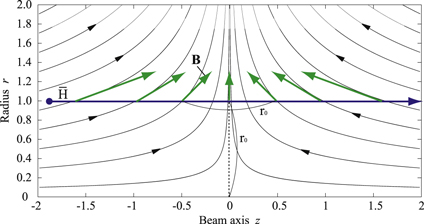
Figure 2. Magnetic field lines of the cusp magnet around the center where the  atom passes through the position z = 0.
Download figure:
Standard image High-resolution imageTrajectories of  atoms in the cusp magnetic field are calculated solving the Newtonian equations of motion numerically. Initial emission directions of
  atoms are assumed to be isotropic. The z component of the magnetic field,
  , of the model cusp magnet is drawn in figure 3(a). Figures 3(b) and (c) show examples of trajectories of
  atoms in ground states having the initial kinetic energy of
  K synthesized at the maximum magnetic field,
  T, for LFS and HFS, respectively (
 is given as a temperature unit, i.e., the kinetic energy divided by Boltzmannʼs constant). It is seen that the number of
  atoms in LFS traveling along the magnet axis is much larger than that in HFS; i.e., one can obtain an intensified and spin-polarized
  beam automatically. The 10 cm disk 1.5 m downstream from the cusp magnet center actually corresponds to the size and the position of the entrance of the microwave cavity in the ASACUSA setup (see figure 1).

Figure 3. (a) The z component of the magnetic field,  , of the model cusp magnet. (b) Trajectories of
  atoms in LFS synthesized on the magnet axis at the maximum magnetic field
  having the kinetic energy of
  K. The open circle in (b) shows the
  production position. The disk with its diameter of 10 cm placed at z = 1.5 m shows the size and the position of the entrance of the ASACUSA microwave cavity (see figure 1). Initial emission directions are assumed to be isotropic, and the lines are drawn every 1 degree from the beam axis. (c) The same as (b) but for
  atoms in HFS.
Download figure:
Standard image High-resolution imageFigure 4(a) again shows  . Symbols in figures 4(b) and (c) plot the fractions of LFS (
 ) and HFS (
 )
)  atoms reaching the 10 cm disk, calculated solving the equations of motion as a function of the
  production position,
  , respectively. Different symbols correspond to different kinetic energies,
  , from 5 K to 100 K. The thick blue solid lines in figures 4(b) and (c) show the fraction of
  atoms arriving at the disk when
  atoms are emitted isotropically following straight trajectories (the solid angle divided by
  from
from  to the 10 cm disk). For all the temperatures calculated, the fractions of
  atoms in LFS transported to the disk are larger than the fraction of the straight trajectory case for
  m; i.e.,
  beams in LFS are focused. In the case of
  K and 10 K (the red open circles and blue open diamonds, respectively), the fraction increases considerably for smaller
  . In other words, the best position to synthesize
  atoms is located upstream of the cusp magnet center, although synthesis at the center was anticipated in the original cusp trap scheme [13]. This is particularly true because the densities of antiproton and positron plasmas are higher at the higher magnetic field, resulting in a higher
  yield. Actually, the first
  production in the cusp trap was realized at the maximum magnetic field region taking this optimal property into account [9, 10]. In the case of
  ,
,  reaches its maximum at
  m (with the intensity enhancement of ∼ 200), because 5 K
  atoms produced at
  m are focused on the disk 1.5 m downstream of the cusp magnet. For
  ,
,  is almost constant, independent of
  . This finding suggests that
  atoms in a certain kinetic energy range can be synthesized in a strong magnetic field region, where a well-known nested potential configuration [14] can be applied, still optimizing the
  beam intensity. For
  atoms in HFS in figure 4(c), the behavior is just the opposite: the lower the kinetic energy, the lower the transport efficiency; i.e., the cusp magnetic field acts in itself as the spin filter as well as the beam intensifier of
  atoms in LFS. Figure 4(d) shows the polarization of
  beams calculated using the results of figures 4(b) and (c) assuming that an equal number of LFS and HFS are produced, where the polarization is defined by
  . The polarization decreases gradually as
  increases.

Figure 4. (a)  on axis. The different symbols in (b) and (c) correspond to the calculated transport fraction of
  atoms in LFS and HFS reaching the 10 cm disk, solving the equations of motion as a function of the production position
  . The curves in (b) and (c) correspond to the transport fraction evaluated using equations (1) and (5) (see the text for details), respectively. (d) The spin-polarization of
  atoms reaching the disk.
Download figure:
Standard image High-resolution image3. Lens formula and the scaling law
Having observed that the cusp magnet has the ability to enhance the beam intensity of  atoms in LFS, the next step is to quantitatively study the transport property. In doing so, the image point,
  , is evaluated calculating trajectories with different ejection angles,
  , from the axis at a fixed object point (
 production position
  ). Then, the thin lens formula,
  , is applied to get the focal length l, where a and b are given by
  and
and  , respectively, and
  is an effective lens position. Figure 5(a) shows the example of l evaluated using
  for 10 K
  atoms in LFS produced at
  m assuming
  m for
m for  . It is observed that for different ejection angles, l is distributed in a narrow region for a fixed
  ; i.e., the concept of the focal length is well satisfied. In the following, the central value of l for
  atoms arriving at the disk is re-defined as the focal length l. Figure 5(b) shows l evaluated as a function of
  for 10 K
  atoms (
 ,
,  and
and  ). Figures 5(c) and (d) are the same as figure 5(b) but for
  and 70 K, respectively. It is observed that l can be determined consistently independent of
  for each
  if
if  is chosen to be ∼0.05 m; i.e., the cusp magnet acts practically as a converging lens for
  beams in LFS, fulfilling the lens formula with a small aberration. Figure 5(e) shows l as a function of
  for 5 K
  , setting
  . l is almost constant for
  m for each
  . Figure 5(f) shows l as a function of
  for five different
  with
with  m, where l is evaluated, e.g., from figure 5(e) for
  m in the case of
  T, and the lines are drawn employing the linear least square method. It is seen that l increases linearly with
  , having a steeper slope for a lower
  . Furthermore, all lines merge at the same point when
  is extrapolated to 0 with a finite intercept,
  0.09 m. Figure 5(g) plots
  as a function of
  . All the lines overlap with each other; i.e., l has an excellent scaling property with respect both to
  and to
  :
:

for  atoms in LFS (
 ). Because we know the lens position,
  , as well as l,
  and
and  , the transport fraction of
  atoms to the 10 cm disk is easily calculated, and is shown by the lines in figure 4(b). These lines are in good agreement with results obtained by numerical simulations (symbols in figure 4(b)).
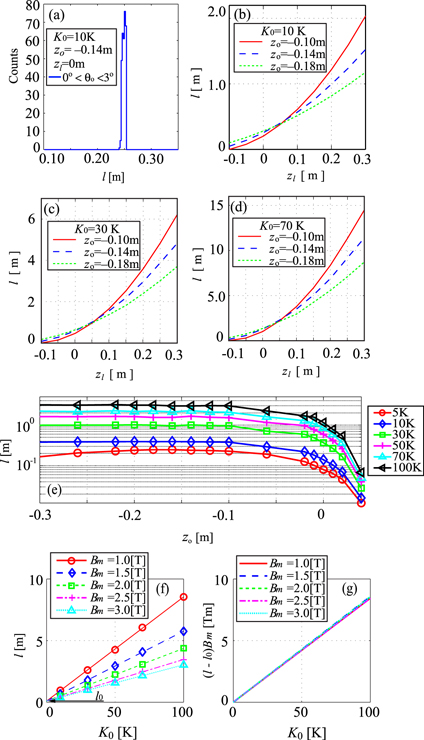
Figure 5. (a) The focal length distribution of  atoms in LFS evaluated using the relation
  for the ejection angle of
  . (b), (c) and (d) The focal length l for
  atoms in LFS as a function of
  for three different
  for
for  , 30 and 70 K. (e) The focal length l as a function of
  for
for  atoms in LFS with
  . (f) The focal length l as a function of
  for
for  atoms in LFS with
  for five different
  . (g)
. (g)  as a function of
  for
for  atoms in LFS with
  .
.
Download figure:
Standard image High-resolution image4. Qualitative analysis of the property of the cusp magnet
To understand why the lens formula is applicable to the cusp magnet, which is quadrupolar in its nature but not sextupolar, the behavior of the magnetic field of the cusp magnet is studied in detail. The focusing property is primarily determined by the radial force acting on the beam; i.e.  for
for  atoms in LFS. Figure 6(a) shows
  , and figure 6(b) is a closeup for 0 m
  m. When
  ,
,  is 0 at r = 0 and increases monotonically with r for
  m (actually the inner radius of the MRE in the ASACUSA setup is 0.04 m). Although
  is almost constant with respect to r at z = 0, this is just a singular point. Taking e.g.
  at z = 0.004 m (the curve closest to z = 0 in figure 6(b)), it increases more or less linearly for
  . As a whole,
  can be practically approximated as
  , where
  is a coefficient of the field gradient as a function of z. Accordingly, the radial force acting on the
  atom is given by
  ; i.e., the cusp magnet here behaves like a sextupole magnet (
 ).
).
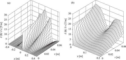
Figure 6. (a)  of the model cusp magnet. (b) The closeup of (a).
Download figure:
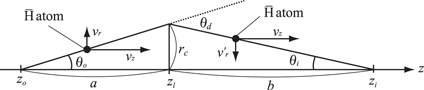
Standard image High-resolution imageThe change of the deflection angle,  , due to the radial momentum transfer from the magnetic field to the
  atom is given by
where m is the  mass,
mass,  and
and  . In contrast to the direction, the radial position of
  atoms does not vary very much during the deflection; therefore the trajectory of
  atoms can be approximated as in figure 7. In this case, the radial position of the
  atom produced at
  with its ejection angle
  with respect to the axis is given by
  at
at  , and the angle at the image point,
  , is given by
  . In this case, all the trajectories meet at the same point at
  , independent of
  . Using a and b above, one can immediately obtain the focal length l as
  . Furthermore, the small correction appearing in equation (1) can be understood as the result of the acceleration of
  atoms in LFS by the magnetic field, which amounts to
  . By replacing
  with
with  , one gets
where  and
and  are the Bohr magneton and Boltzmannʼs constant, respectively. The third equation is obtained considering the size of the magnet (
 ) and
) and 
 assuming
  T/m at r = 0.04 m (figure 6(b)). For the ground state (
 ), equation (4) is semi-quantitatively consistent with equation (1); i.e., the behavior of the cusp magnet is well understood. As shown in equation (3),
  also has the scaling property with respect to μ.
Figure 7. A schematic trajectory of the  atom in LFS approximating that the momentum transfer takes place only at
  .
.
Download figure:
Standard image High-resolution image
In the case of  atoms in HFS, the direction of the force is just the opposite; i.e.,
  atoms are axially decelerated and radially defocused. Accordingly, by replacing
  by
by  and
and  by
by  , and employing more correct coefficients obtained in equation (1), one gets

The transport fraction of  atoms in HFS can be evaluated in a similar way as in LFS, employing equation (5), which is shown by the lines in figure 4(c). It is seen that these lines reproduce the results of numerical simulations quite well. The polarization using
  and
and  is also shown by the lines in figure 4(d), which again reproduces the numerical simulations quite well; i.e., the cusp magnet works as a magnetic lens for LFS and also for HFS
  beams. It is also noted that the cusp magnet can be used as a good spin-selector for molecular beam experiments.
5. Conclusion
Here, we study the transport properties of cold  atoms produced in the cusp magnet. Although the cusp magnet (anti-Helmholtz coils) has in principle a quadrupolar field distribution, it is found that the
  beams prepared upstream of the center of the cusp magnet are well characterized and follow the lens formula of optical lenses. The focal length satisfies a scaling law on the initial kinetic energy (
 ), the maximum magnetic field strength(
 ) and the magnetic moment (μ) of
  atoms. Because the cusp magnet focuses
  atoms in LFS along the magnet axis and defocuses those in HFS, one gets a spin-polarized intensified
  beam automatically.
Furthermore, it is found that the best position to produce  atoms for a stronger
  beam with higher polarization is upstream of the center of the cusp magnet for a broad range of
  kinetic energy. This allows the use of the so-called nested trap configuration, which greatly simplifies the
  production procedures.