


Abstract
We derived the effective Hamiltonians for silicene and phosphorene with strain, electric field and magnetic field using the method of invariants. Our paper extends the work of Geissler et al 2013 (New J. Phys. 15 085030) on silicene, and Li and Appelbaum 2014 (Phys. Rev. B 90, 115439) on phosphorene. Our Hamiltonians are compared to an equivalent one for graphene. For silicene, the expression for band warping is obtained analytically and found to be of different order than for graphene. We prove that a uniaxial strain does not open a gap, resolving contradictory numerical results in the literature. For phosphorene, it is shown that the bands near the Brillouin zone center only have terms in even powers of the wave vector. We predict that the energies change quadratically in the presence of a perpendicular external electric field but linearly in a perpendicular magnetic field, as opposed to those for silicene which vary linearly in both cases. Preliminary ab initio calculations for the intrinsic band structures have been carried out in order to evaluate some of the  parameters.
Export citation and abstract BibTeX RIS

Content from this work may be used under the terms of the Creative Commons Attribution 3.0 licence. Any further distribution of this work must maintain attribution to the author(s) and the title of the work, journal citation and DOI.
1. Introduction
Graphene is an interesting electronic material because of its two-dimensionality, zero-gap, and linear dispersion near the Fermi energy [1]. These properties differ from standard three-dimensional semiconductors. The study of other two-dimensional materials beyond graphene came about quickly, with BN and MoS2 being two early choices. More recent candidates include silicene [2] and phosphorene [3], though earlier studies of these two materials exist [4, 5].
Nowadays, much of the study of electronic properties relies on ab initio calculations, in particular density-functional theory (DFT). DFT is very powerful in its ability to predict ground-state properties such as structures fairly well. It is less reliable and much more computationally intensive to calculate excited-state properties such as optical and transport properties; the inclusion of an external magnetic field is still a difficult problem and not implemented in standard DFT codes. Empirical tight-binding models have been early alternatives to DFT; indeed, the linear dispersions for both graphene [6] and silicene [2] were first identified using tight-binding models, even though the linear dispersion for silicene was probably first obtained (but not identified) in 1994 using ab initio calculations [4].
However, the most versatile and physically-transparent band-structure model is the  model [7], often giving energy bands analytically in the vicinity of extrema in terms of meaningful parameters such as effective masses and optical matrix elements. For graphene, this is the Dirac Hamiltonian linear in the wave vector, though nonlinear contributions have also been worked out [8]. For silicene, only the Dirac Hamiltonian, with linear electric field terms, has been written down [9]. For phosphorene, a couple of
  models have recently appeared [10, 11]. Li and Appelbaum [11], in particular, did a very careful study of the band structure using perturbation theory near the Γ point, identifying the contributions to the effective masses; however, they again did not include external fields.
In the current work, we are therefore concerned with the most general  Hamiltonian for silicene and phosphorene, particularly in the presence of external fields since this problem has not been considered fully. We employ the method of invariants to derive such Hamiltonians. The primary goal is to identify possible terms not considered in previous work. A secondary goal is to thus obtain a better understanding of the band structures of silicene and phosphorene.
2. Method of invariants
Here we apply the method of invariants [12] to the materials of interest to us. Since most of the DFT calculations to date have not included relativistic effects and we are considering low atomic number elements, we have left out spin effects in this work; the main consequence in the band structure is the neglect of the small spin–orbit splitting of bands (e.g., for silicene, this is a 1.55 meV splitting at the K point [13]). The symmetries of interest are the space-group symmetries and time-reversal symmetry. Space-group symmetry only requires one to study the character tables of the point-group symmetry, whereas the consideration of time-reversal symmetry requires an application of the Herring test [12]. Details of the theory are not repeated here as we have applied the formalism exactly as presented in [12].
2.1. Silicene
The point of interest for silicene is the K point in the first Brillouin zone (figure 1) since that is where the valence and conduction bands touch with a linear dispersion. In table 1, the group of the wave vector at point K for silicene is shown. We use the expressions

and similarly for other physical quantities. It can be seen that all the irreducible representations are either one-dimensional or two-dimensional, implying that the energy bands at K are all either non-degenerate or doubly degenerate. The Fermi level is at a point of double degeneracy.
Table 1.
Group of wave vector D3 at the K point (silicene). ki are components of the wave vector,  of the strain tensor, Bi of an external magnetic field, Ei of an external electric field, and
  of an angular momentum operator.
| D3 | E | 2C3 |

|
Odd | Even | Matrix |
|---|---|---|---|---|---|---|

|
1 | 1 | 1 |

|

|
|

|
1 | 1 | −1 |

|
Ez |

|

|
2 | −1 | 0 |

|

|

|
Table 2. D3 multiplication table of irreducible representations.

|

|

|
|
|---|---|---|---|

|

|

|

|

|

|

|

|

|

|

|

|
Table 3.
D3 coupling constant table ( ). The notations
  and
and  denote the first component of the first
  function and the second component of the second
  function, respectively, etc.

|
|
|---|---|
 : : |

|
 : : |

|
 : : |

|
 : : |

|
Tables 1–3 allow us to determine the Hamiltonian from combinations of single group functions based on symmetry principles formed. The next step is to apply the Herring test [12]. It follows from the character table of D3 that

for all representations  where n = 6 is the order of the group D3, g is a representation of a group element, and χ is the character of that group element. Further, since a spatial symmetry
  exists such that
  where
where  is the K point (and
  ), all irreducible representations belong to the case a2 [12]. In this case, time-reversal symmetry additionally requires all Hamiltonian terms to satisfy

where  ,
,  , and
, and  are the time-reversal operator, a
  invariant term, and a spatial symmetry operator establishing a link between basis functions at
  and
and  , respectively. In the case of silicene,
  and
and  can be chosen where
  denotes reflection in the x axis using a coordinate system where the x axis passes through the center of an edge in the honeycomb lattice formed by the silicon atoms (referring to the same choice of coordinate system as in [14]). The symbol ζ takes the value +1 and −1 for even and odd functions under time-reversal symmetry, respectively.
With the preceding analysis, we can write down the most general Hamiltonian for silicene allowed by symmetry. The result is, to leading orders,


where the dots refer to higher-order terms. ai, bi, ci and ei are  parameters which are undetermined in the method of invariants. The Hi terms are intrinsic band-structure Hamiltonians while the other ones exist in the presence of external fields. In the above Hamiltonian, the
  matrices represent the pseudospin degree of freedom and are the
  Pauli spin matrices. The difference between the work of Geissler et al [9] and the current one is that they were focussed on the interplay between spin–orbit coupling and an external electric field (and, hence, in the topological properties) at the linear level (in k and Ez), whereas we are more interested in understanding the basic band structure of the material beyond the linear terms and in the presence of other external fields. Thus, the a2 and a3 terms provide quadratic in k contributions while the a4 and a5 are of cubic order but only the a4 term gives rise to an anisotropic term. Hence, one can readily say that the band structure of silicene to linear and quadratic orders is isotropic and anisotropic effects only manifest themselves if cubic terms become important. A discussion of the band dispersion is provided in the next section.
For comparison, we reproduce the corresponding  for graphene [8]:

The sign difference in the a61 term is due to a different choice of phase while the a62 is the corresponding anisotropy term for graphene. It is seen here to be quadratic in k though it is cubic in k for silicene.
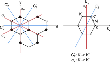
Figure 1. Real (left) and reciprocal (right) space pictures of the structure of silicene. The two atoms (solid and open circles) are at different vertical heights.
Download figure:
Standard image High-resolution image2.2. Phosphorene
Phospherene and its bulk counterpart black phosphorus have the same in-plane translational symmetry and the nonsymmorphic space group is base-centered orthorhombic [11] (figure 2). Its factor group is symmorphic with  whose character table and associated functions are shown in table 4.

Figure 2. Real (left) and reciprocal (right) space pictures of the structure of phosphorene. The two atoms (solid and open circles) are at different vertical heights.
Download figure:
Standard image High-resolution imageTable 4.
Group of wave vector  at the Γ point (phosphorene).

|
E |

|

|

|
i |

|

|

|
Odd | Even | Matrix |
|---|---|---|---|---|---|---|---|---|---|---|---|

|
1 | 1 | 1 | 1 | 1 | 1 | 1 | 1 |

|

|
|

|
1 | −1 | 1 | −1 | 1 | −1 | 1 | −1 | By |

|

|

|
1 | 1 | −1 | −1 | 1 | 1 | −1 | −1 | Bz |

|

|

|
1 | −1 | −1 | 1 | 1 | −1 | −1 | 1 | Bx |

|

|

|
1 | 1 | 1 | 1 | −1 | −1 | −1 | −1 | |||

|
1 | −1 | 1 | −1 | −1 | +1 | −1 | 1 | ky | Ey | |

|
1 | 1 | −1 | −1 | −1 | −1 | 1 | 1 | kz | Ez | |

|
1 | −1 | −1 | 1 | −1 | 1 | 1 | −1 | kx | Ex |
The multiplication table of irreducible representations for  is given in table 5. Note that the parity of the product representation follows the simple rule:
  ,
,  ,
,  ,
,  etc. Since the irreducible representations are all one-dimensional, the coupling constants of product representations are trivial. Further, since
  at the Γ point and the condition in equation (2) is satisfied by the irreducible representations, all irreducible representations belong to the case a1 [12].
Table 5.
 multiplication table of irreducible representations.

|

|

|

|
|
|---|---|---|---|---|

|

|

|

|

|

|

|

|

|

|

|

|

|

|

|

|

|

|

|

|
We are now in a position to write down the most general Hamiltonian for phospherene allowed by symmetry. The result is


Our intrinsic Hamiltonian agrees with the result of Li and Appelbaum [11].
3. Band structures
We now provide some discussion of the band structures that can be inferred from the Hamiltonians. We are also more interested in revealing the properties analytically than purely numerically using DFT calculations. However, preliminary calculations of the intrinsic band structures have been performed. The DFT-based calculations were conducted using the projector augmented-wave method [15] and the PBE–GGA exchange-correlation functional [16] as implemented in the VASP code [17–19]. The electronic wavefunctions were described using a plane-wave basis set with an energy cutoff of 500 eV for silicene and 1200 eV for phosphorene. Atomic positions were fully relaxed in Γ-centered 25 × 25 × 1 for silicene (9 × 9 × 1 for phosphorene) supercells for k-point sampling until residual forces were lower than 5 meV Å−1. For silicene, the lattice constant obtained was 3.867 Å. For phosphorene, the optimized lattice constants were 3.300 and 4.624 Å. In both cases, a large interlayer separation in the z direction was chosen ( Å) to minimize interactions.
3.1. Silicene
We are mainly concerned with the doubly-degenerate Dirac band since the Fermi level crosses it; it is made of pz and s orbitals from both atoms in the unit cell of silicene [2].
3.1.1. Intrinsic
For an arbitrary direction and keeping terms up to cubic in k, the band structure is given by diagonalizing the Hi Hamiltonian. Writing  , one gets

Thus, our equation above shows that the intrinsic band dispersion can have quadratic, cubic, ... terms in the wave vector.
The a1 coefficient is related to the Fermi velocity, a2 is related to an effective mass, a4 gives rise to anisotropy, and a5 leads to cubic terms. Along the  direction (ky = 0), the band structure simplifies to

This reproduces the well-known result for graphene that the Fermi speed is the same for the two bands (figure 3, left). Note that the anisotropy parameter a4 is absent along this direction.
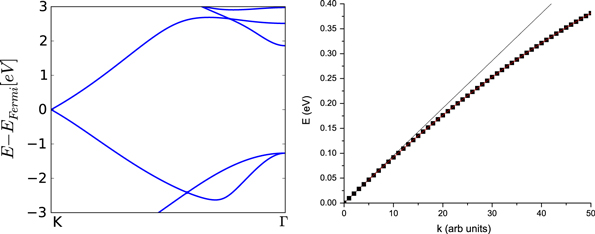
Figure 3. Left: band dispersion for silicene along the K to Γ direction. Right: band dispersion for silicene along the K to M/2 direction. The black line is keeping only the linear term.
Download figure:
Standard image High-resolution imageWe have performed a cubic fit of the bands obtained using VASP up to about half-way from K. Rewriting equation (19) as

and performing a fit to

where n is chosen to be 100 points between K and G, we obtain (with  )
)


and where we have used  Å.
Å.
The results of the curve fitting are given in table 6.
Table 6. Band fitting for silicene along K to Γ.
| B1 | vF ( ) ) |
B2 |

|
B3 |

|
|
|---|---|---|---|---|---|---|
| VB | −0.040 | 6.43 |

|
−0.66 |

|
6.65 |
| CB | 0.035 | 5.63 |

|
0.36 |

|
−8.51 |
Figure 3 (right) shows the dispersion along  (symbols). It can be seen that the linear dispersion (line) is a good approximation only up to about a third of the way.
3.1.2. Strain
In the presence of strain, the Hamiltonian at the K point is given by

First, we note that applying strain perpendicular to the plane ( ) does not change the symmetry at the K point and a zero gap is preserved but there is nevertheless an expected shift in the energy levels. Second, an in-plane uniaxial strain (e.g.,
  ), while changing the symmetry, leads to the same energy change for both bands making up the Dirac point since they both have the same deformation potential e1; thus, the only effect is a shift in energies. Our analysis provides a formal resolution to the controversy from DFT calculations about whether a gap is opened by a uniaxial strain or not [20–23]. Zhao and Mohan et al both predicted a gap opening [20, 21]. However, Qin et al [24] and Yang et al [23] did not obtain a gap and only obtained a shift of the Dirac point. The latter interpreted the disagreement of Zhao to their using insufficient k points near the crossing. However, the influence of strain does significantly change the dispersion at finite k values, i.e., in the Fermi velocity of those bands.
For finite k and an arbitrary strain, one can also diagonalize the Hamiltonian to give


3.1.3. Electric field
In the presence of an electric field, the Hamiltonian at the K point is given by

An electric field in the z-direction will change the symmetry for silicene (as opposed to graphene which has all the atoms in the plane) and, therefore, a gap will open. Earlier DFT calculations have shown that the gap opening is initially linear in the field (hence  ) and later becomes nonlinear. This behaviour is reproduced by our symmetry analysis. Indeed, by comparing to the DFT calculations of Drummond et al [25], one obtains
  eÅ. No existing calculations allow us to determine c2 and c3.
In figure 4 (left), dispersion plots are shown near the K point for an applied electric field Ey = 1 (top, in arbitrary units) and for  (bottom, in arbitrary units). Note that the plots are relative energies as they do not include the solution of the equations in the y direction which requires numerically solving the Airy equation.

Figure 4. Left: two plots of dispersion relations near the K point for an applied electric field using the expression for  in equation (8) and linear in k. Parameter values are in arbitrary units: (top)
  ; (bottom)
  . Right: the same with magnetic field instead: (top)
  ; (bottom)
  .
.
Download figure:
Standard image High-resolution image3.1.4. Magnetic field
Finally, we present the behaviour of the energies in the presence of a magnetic field. First, the Hamiltonian linear in the magnetic field is

Thus, at the K point, we have

Similarly to the electric field case, the magnetic-field problem is separable and only the soluble part is plotted in figure 4.
3.2. Phosphorene
For phospherene, since the irreducible representations are all one dimensional, the Hamiltonians are the same as the dispersion relations. Thus, the band structure is simpler to interpret. From equation (13), it can be seen that (in the absence of spin–orbit interaction), only terms in even powers of ki are allowed. There is also an obvious anisotropy in the effective mass due to the orthorhombic symmetry.
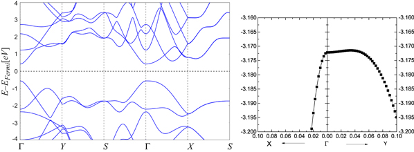
Our DFT calculations (figure 5) are consistent with others already published (e.g., [3, 10]). The gap is almost direct at the Γ point and the GGA value is about 0.98 eV; Tran et al [26] have shown that a GW correction increases the gap to 2.0 eV. We performed a fit to our DFT calculations (table 7).
Figure 5. Band structure of phosphorene. On the right is a close up of the highest valence band near the Γ point.
Download figure:
Standard image High-resolution image
Table 7. Effective masses (in units of m0) of the highest valence and lowest conduction bands of phosphorene at the Γ point. The effective mass of the VB along ΓY is very sensitive to the computation.
| Γ Y | ΓX | |
|---|---|---|
| CB | 1.24 | 0.173 |
| 1.246 [27], 1.16 [28] | 0.146 [27], 0.22 [28] | |
| VB | 7.2 | −0.160 |
| 3.24 [28] | −0.19 [28] |
While early calculations reported phosphorene to be a direct-gap semiconductor [3, 5], subsequent calculations have revealed it to be slightly indirect [10, 11, 29] with an almost flat dispersion in the ΓY direction. An interesting observation is the fact that some bands merge along the surface of the Brillouin zone, leading to double degeneracy (even though the character tables of the group of wave vector only reveal one-dimensional irreducible representations). The origin of the band sticking is the nonsymmorphic nature of the space group [30].
3.2.1. Strain
We note that a number of DFT calculations of strained phosphorene have recently been reported [27–29, 31, 32], though all for large strains up to  %. The leading terms in the strain Hamiltonian are

At the Γ point, the energies are

where Ei are the band edges in the absence of strain. Contrary to the case for silicene, now a uniaxial strain in any of the directions or a biaxial strain will change the size of the band gap if the deformation potentials for different bands are different. The particular case of a perpendicular strain has recently been modeled by compressing the atoms within the unit cell in a DFT calculation and shown to lead to a possible semiconductor-metal transition [10]. Fei et al [27] found that a biaxial strain (about 4%) or a zigzag uniaxial strain (between 5 and 6%) can change the order of the lowest two conduction bands.
For a finite wave vector, the total one-dimensional Hamiltonian is


3.2.2. Electric field
We note that, in contrast to both graphene and silicene, equation (15) shows that the band energies change quadratically with an externally-applied electric field. At k = 0, the band energies for a perpendicular field are

DFT results just published appear to confirm our prediction [28].
3.2.3. Magnetic field
In an external magnetic field, the one-band problem is exactly solvable in terms of the standard Landau level problem. Thus, with a static magnetic field  with a vector potential
  , the Hamiltonian is given by [7]

The eigenfunctions can be separated,

and the eigenvalues are equidistant Landau levels

where  . Thus, the prediction is that, to the lowest order, a perpendicular magnetic field will change the energy levels linearly.
4. Summary
The method of invariants was used to obtain analytical forms for the Hamiltonians and band structures of silicene and phosphorene beyond the lowest order terms and in the presence of external fields. Differences in the band structures of graphene, silicene and phosphorene are pointed out. Our method provides a formal analysis that is not possible from ab initio calculations. Specifically, some of the main conclusions derived from the theory include
- anisotropy in the band structure of silicene shows up at the cubic order whereas they show up at the quadratic level for graphene.
- an in-plane uniaxial strain does not open a gap for silicene.
- a perpendicular strain does not open a gap for silicene but would change the gap for phosphorene.
- to the lowest-order the energies levels of silicene change linearly with an external magnetic field and a perpendicular electric field, whereas, for phosphorene, the energy levels change quadratically with a perpendicular electric field and linearly with a perpendicular magnetic field.
Ab initio calculations for the intrinsic band structures are included and more extensive calculations with external perturbations will be reported in a future publication.
Acknowledgments
LLYV acknowledges the support of the Traubert Chair. Work at Argonne is supported by DOE-BES under contract no. DE-AC02–06CH11357; ALB acknowledges Glue funding from DOE (FWP#70081). MW would like to thank The Citadel for travel support. YZ acknowledges the support of the Bissell Distinguished Professorship.