Interlayer interaction in general incommensurate atomic layers

Recently there have been extensive research efforts on atomically-thin nanomaterials, including graphene, hexagonal boron nitride (hBN), phosphorene and the metal transition dichalcogenides. The hybrid systems composed of different kind of atomic layers have also attracted much attention, and there the interaction at the interface between the different atomic layers often plays an important role in the physical property. In such a composite system, the lattice periods of the individual atomic layers are generally incommensurate due to the difference in the crystal structure and also due to misorientation between the adjacent layers. A well-known example of irregularly stacked multilayer system is the twisted bilayer graphene, in which two graphene layers are rotationally stacked at an arbitrary angle [1]. When the rotation angle is small, in particular, the system exhibits a moiré interference pattern of which period can be much greater than the atomic scale, and such a long-period modulation is known to strongly influence the low-energy electronic motion [2–14]. Graphene–hBN composite system has also been intensively studied as another example of incommensurate multilayer system, where the two layers share the same hexagonal lattice structure but with slightly-different lattice constants, leading to the long-period modulation even at zero rotation angle [15–21]. The electronic structure in graphene–hBN system was theoretically studied [22–35], and the recent transport measurements revealed remarkable effects such as the formation of mini-Dirac bands and the fractal subband structure in magnetic fields [18–20, 36].

The previous theoretical works mainly targeted the honeycomb lattice to model twisted bilayer graphene and graphene–hBN system, and also particularly focus on the long-period moiré modulation which arises when the crystal structures of two layers are slightly different. Then we may ask how to treat general bilayer systems where the lattice vectors of the adjacent layers are not close to each other. In this paper, we develop a theoretical formulation to describe the interlayer interaction effect in general bilayer systems with arbitrary choice of crystal structures and relative orientations. By starting from the tight-binding model with the distance-dependent transfer integral, we show that the interlayer coupling can be simply written in terms of a generalized Umklapp process in the reciprocal space. We then apply the method to the incommensurate bilayer graphene with a large rotation angle (θ = 20°) which cannot be treated as a long-range moiré superlattice, and obtain the quasi band structure and density of states within the first-order approximation. Finally, we apply the formulation to the moiré superlattice where the two lattice structures are close, and demonstrate that the long-range effective theory is naturally derived.

We consider a bilayer system composed of a pair of two-dimensional atomic layers having generally different crystal structures as shown in figure 1. We write the primitive lattice vectors as ${{{\bf a}}_{1}}$ and ${{{\bf a}}_{2}}$ for layer 1 and ${{\tilde{{\bf a}}}_{1}}$ and ${{\tilde{{\bf a}}}_{2}}$ for layer 2, which are all along in-plane (x−y) direction. The reciprocal lattice vectors are defined by ${{{\bf G}}_{i}}$ and ${{\tilde{{\bf G}}}_{i}}$ for layers 1 and 2, respectively, so as to satisfy ${{{\bf a}}_{i}}\cdot {{{\bf G}}_{j}}={{\tilde{{\bf a}}}_{i}}\cdot {{\tilde{{\bf G}}}_{j}}=2\pi {{\delta }_{ij}}$. The area of the unit cell is given by $S=\mid {{{\bf a}}_{1}}\times {{{\bf a}}_{2}}\mid$ and $\tilde{S}=\mid {{\tilde{{\bf a}}}_{1}}\times {{\tilde{{\bf a}}}_{2}}\mid$ for layers 1 and 2, respectively. Without specifying any details of the model, we can easily show that an electronic state with a Bloch wave vector ${\bf k}$ on layer 1 and one with $\tilde{{\bf k}}$ on layer 2 are coupled only when

$$\begin{eqnarray}&&{\bf k}+{\bf G}=\tilde{{\bf k}}+\tilde{{\bf G}},\end{eqnarray} \tag{ 1 }$$

where ${\bf G}={{m}_{1}}{{{\bf G}}_{1}}+{{m}_{2}}{{{\bf G}}_{2}}$ and $\tilde{{\bf G}}={{\tilde{m}}_{1}}{{\tilde{{\bf G}}}_{1}}+{{\tilde{m}}_{2}}{{\tilde{{\bf G}}}_{2}}$ are reciprocal lattice vectors of layers 1 and 2, respectively. This is regarded as a generalized Umklapp process between arbitrary misoriented crystals, and it can be easily understood by considering the wave decomposition in the plain wave basis as follows. A Bloch state on layer 1 (say $\phi _{{\bf k}}^{(1)}$) is expressed as a summation of ${{{\rm e}}^{{\rm i}({\bf k}+{\bf G})}}$ over the reciprocal vectors ${\bf G}$, and one on layer 2 ($\phi _{\tilde{{\bf k}}}^{(2)}$) is expressed as a summation of ${{{\rm e}}^{{\rm i}(\tilde{{\bf k}}+\tilde{{\bf G}})}}$ over $\tilde{{\bf G}}$. Also, Hamiltonian of the total system consists of Fourier components of ${\bf G}$ and $\tilde{{\bf G}}$. As a result, the matrix element $\langle \phi _{\tilde{{\bf k}}}^{(2)}\mid H\mid \phi _{{\bf k}}^{(1)}\rangle$ can be non-zero only under the condition equation (1).

Zoom In Zoom Out Reset image size

In the following, we actually calculate the matrix elements for generalized Umklapp processes using the tight-binding model. We assume that a unit cell in each layer contains several atomic orbitals, which are specified by X = A, B, ⋯ for layer 1 and $\tilde{X}=\tilde{A},\tilde{B},\cdots$ for layer 2. The lattice positions are given by

$$\begin{eqnarray}\begin{array}{rcl} {{{\bf R}}_{X}} & = & {{n}_{1}}{{{\bf a}}_{1}}+{{n}_{2}}{{{\bf a}}_{2}}+{{{\boldsymbol{ \tau }} }_{X}}\qquad \qquad \qquad \qquad ({\rm layer}\ 1), \\ {{{\bf R}}_{\tilde{X}}} & = & {{\tilde{n}}_{1}}{{\tilde{{\bf a}}}_{1}}+{{\tilde{n}}_{2}}{{\tilde{{\bf a}}}_{2}}+{{{\boldsymbol{ \tau }} }_{\tilde{X}}}\qquad \qquad \qquad \qquad ({\rm layer}\ 2), \\ \end{array}\end{eqnarray} \tag{ 2 }$$

where n_i and ${{\tilde{n}}_{i}}$ are integers, and ${{{\boldsymbol{ \tau }} }_{X}}$ and ${{{\boldsymbol{ \tau }} }_{\tilde{X}}}$ are the sublattice position inside the unit cell, which can have in-plane and out-of-plane components. When the atomic layers are completely planar and stacked with interlayer spacing d, for instance, we have ${{{\boldsymbol{ \tau }} }_{X}}\cdot {{{\bf e}}_{z}}=0$ for layer 1 and ${{{\boldsymbol{ \tau }} }_{\tilde{X}}}\cdot {{{\bf e}}_{z}}=d$ for layer 2, where ${{{\bf e}}_{z}}$ is the unit vector in z-direction.

Let us define $\mid {{{\bf R}}_{X}}\rangle \equiv {{\phi }_{X}}({\bf r}-{{{\bf R}}_{X}})$ as the atomic state of the sublattice X localized at ${{{\bf R}}_{X}}$. The atomic orbital ${{\phi }_{X}}$ may be different depending on X. We assume the transfer integral from the site ${{{\bf R}}_{X}}$ to ${{{\bf R}}_{\tilde{X}}}$ is written as $-{{T}_{\tilde{X}X}}({{{\bf R}}_{\tilde{X}}}-{{{\bf R}}_{X}})$, i.e., depending on the relative position ${{{\bf R}}_{\tilde{X}}}-{{{\bf R}}_{X}}$ and also on the sort of atomic orbitals of X and $\tilde{X}$. The interlayer Hamiltonian to couple the layers 1 and 2 is then written as

$$\begin{eqnarray}&&U=-\mathop{\sum }\limits_{X,\tilde{X}}{{T}_{\tilde{X}X}}({{{\bf R}}_{\tilde{X}}}-{{{\bf R}}_{X}})\mid {{{\bf R}}_{\tilde{X}}}\rangle \langle {{{\bf R}}_{X}}\mid +{\rm h}{\rm .c}..\end{eqnarray} \tag{ 3 }$$

When the superlattice period is huge, constructing Hamiltonian in the real space bases becomes hard because it requires the relative inter-atom position for every single combination of the atomic sites of layers 1 and 2. On the other hand, the interlayer coupling is described in a simpler manner in the reciprocal space. We define the Bloch basis of each layer as

$$\begin{eqnarray}\begin{array}{rcl} \mid {\bf k},X\rangle & = & \frac{1}{\sqrt{N}}\mathop{\sum }\limits_{{{{\bf R}}_{X}}}{{{\rm e}}^{{\rm i}{\bf k}\cdot {{{\bf R}}_{X}}}}\mid {{{\bf R}}_{X}}\rangle \qquad \qquad \qquad \qquad ({\rm layer}\ 1), \\ \mid \tilde{{\bf k}},\tilde{X}\rangle & = & \frac{1}{\sqrt{\tilde{N}}}\mathop{\sum }\limits_{{{{\bf R}}_{\tilde{X}}}}{{{\rm e}}^{{\rm i}\tilde{{\bf k}}\cdot {{{\bf R}}_{\tilde{X}}}}}\mid {{{\bf R}}_{\tilde{X}}}\rangle \qquad \qquad \qquad \qquad ({\rm layer}\ 2), \\ \end{array}\end{eqnarray} \tag{ 4 }$$

where ${\bf k}$ and $\tilde{{\bf k}}$ are the two-dimensional Bloch wave vectors parallel to the layer, $N(\tilde{N})$ is the number of unit cell of layer 1(2) in the total system area ${{S}_{{\rm tot}}}$. Although the layers 1 and 2 are generally incommensurate, we assume the system has a large but finite area ${{S}_{{\rm tot}}}=NS=\tilde{N}\tilde{S}$ to normalize the wave function. Then we can show that the matrix elements of U between Bloch bases can be written as

$$\begin{eqnarray}\begin{array}{rcl} {{U}_{\tilde{X}X}}(\tilde{{\bf k}},{\bf k}) & \equiv & \langle \tilde{{\bf k}},\tilde{X}\mid U\mid {\bf k},X\rangle \\ {} & = & -\mathop{\sum }\limits_{{\bf G},\tilde{{\bf G}}}{{t}_{\tilde{X}X}}({\bf k}+{\bf G}){{{\rm e}}^{-{\rm i}{\bf G}\cdot {{\tau }_{X}}+{\rm i}\tilde{{\bf G}}\cdot {{\tau }_{\tilde{X}}}}}{{\delta }_{{\bf k}+{\bf G},\tilde{{\bf k}}+\tilde{{\bf G}}}}, \\ \end{array}\end{eqnarray} \tag{ 5 }$$

which is non-zero only when the generalized Umklapp condition equation (1) is satisfied. Here $t({\bf q})$ is the in-plane Fourier transform of the transfer integral defined by

$$\begin{eqnarray}&&{{t}_{\tilde{X}X}}({\bf q})=\frac{1}{\sqrt{S\tilde{S}}}\int {{T}_{\tilde{X}X}}({\bf r}+{{z}_{\tilde{X}X}}{{{\bf e}}_{z}}){{{\rm e}}^{-{\rm i}{\bf q}\cdot {\bf r}}}{{{\rm d}}^{2}}r,\end{eqnarray} \tag{ 6 }$$

where ${{z}_{\tilde{X}X}}=({{{\boldsymbol{ \tau }} }_{\tilde{X}}}-{{{\boldsymbol{ \tau }} }_{X}})\cdot {{{\bf e}}_{z}}$, and the integral in ${\bf r}$ is taken over the two-dimensional space of ${{S}_{{\rm tot}}}$. ${\bf G}$ and $\tilde{{\bf G}}$ run over all the reciprocal lattice vectors of layers 1 and 2, respectively. Since ${{t}_{\tilde{X}X}}({\bf k})$ decays in large k, we only have a limited number of relevant components in the summation of equation (5).

Equation (5) is derived in a straightforward manner as follows. By inserting U in equation (3) to the definition of ${{U}_{\tilde{X}X}}$, we have

$$\begin{eqnarray}\begin{array}{rcl} {{U}_{\tilde{X}X}}(\tilde{{\bf k}},{\bf k}) & = & -\frac{1}{\sqrt{N\tilde{N}}}\mathop{\sum }\limits_{{{{\bf R}}_{X}},{{{\bf R}}_{\tilde{X}}}}{{T}_{\tilde{X}X}}({{{\bf R}}_{\tilde{X}}}-{{{\bf R}}_{X}}){{{\rm e}}^{{\rm i}{\bf k}\cdot {{{\bf R}}_{X}}-{\rm i}\tilde{{\bf k}}\cdot {{{\bf R}}_{\tilde{X}}}}}, \\ {} & = & -\frac{1}{\sqrt{N\tilde{N}}}\mathop{\sum }\limits_{{{{\bf R}}_{X}}}{{{\rm e}}^{{\rm i}({\bf k}-\tilde{{\bf k}})\cdot {{{\bf R}}_{X}}}}\mathop{\sum }\limits_{{{{\bf R}}_{\tilde{X}}}}{{T}_{\tilde{X}X}}({{{\bf R}}_{\tilde{X}}}-{{{\bf R}}_{X}}){{{\rm e}}^{-{\rm i}\tilde{{\bf k}}\cdot ({{{\bf R}}_{\tilde{X}}}-{{{\bf R}}_{X}})}}. \\ \end{array}\end{eqnarray} \tag{ 7 }$$

By applying the inverse Fourier transform of equation (6),

$$\begin{eqnarray}&&{{T}_{\tilde{X}X}}({\bf r}+{{z}_{\tilde{X}X}}{{{\bf e}}_{z}})=\frac{1}{\sqrt{N\tilde{N}}}\int {{t}_{\tilde{X}X}}({\bf q}){{{\rm e}}^{{\rm i}{\bf q}\cdot {\bf r}}}{{{\rm d}}^{2}}q,\end{eqnarray} \tag{ 8 }$$

to equation (7), the second summation is transformed as

$$\begin{eqnarray}&&\begin{array}{l} \mathop{\sum }\limits_{{{{\bf R}}_{\tilde{X}}}}{{T}_{\tilde{X}X}}({{{\bf R}}_{\tilde{X}}}-{{{\bf R}}_{X}}){{{\rm e}}^{-{\rm i}\tilde{{\bf k}}\cdot ({{{\bf R}}_{\tilde{X}}}-{{{\bf R}}_{X}})}} \\ \quad =\frac{1}{\sqrt{N\tilde{N}}}\int {{{\rm d}}^{2}}q\;{{{\rm e}}^{{\rm i}({\bf q}-\tilde{{\bf k}})\cdot ({{\tau }_{\tilde{X}}}-{{{\bf R}}_{X}})}}{{t}_{\tilde{X}X}}({\bf q})\mathop{\sum }\limits_{{{\tilde{n}}_{1}}{{\tilde{n}}_{2}}}{{{\rm e}}^{{\rm i}({\bf q}-\tilde{{\bf k}})\cdot ({{\tilde{n}}_{1}}{{\tilde{{\bf a}}}_{1}}+{{\tilde{n}}_{2}}{{\tilde{{\bf a}}}_{2}})}} \\ \quad =\sqrt{\frac{\tilde{N}}{N}}\mathop{\sum }\limits_{\tilde{{\bf G}}}{{t}_{\tilde{X}X}}(\tilde{{\bf k}}+\tilde{{\bf G}}){{{\rm e}}^{{\rm i}\tilde{{\bf G}}\cdot ({{\tau }_{\tilde{X}}}-{{{\bf R}}_{X}})}}, \\ \end{array}\end{eqnarray} \tag{ 9 }$$

where we used in the last equation

$$\begin{eqnarray}&&\mathop{\sum }\limits_{{{\tilde{n}}_{1}}{{\tilde{n}}_{2}}}{{{\rm e}}^{{\rm i}({\bf q}-\tilde{{\bf k}})\cdot ({{\tilde{n}}_{1}}{{\tilde{{\bf a}}}_{1}}+{{\tilde{n}}_{2}}{{\tilde{{\bf a}}}_{2}})}}=\tilde{N}\mathop{\sum }\limits_{\tilde{{\bf G}}}{{\delta }_{{\bf q}-\tilde{{\bf k}},\tilde{{\bf G}}}}.\end{eqnarray} \tag{ 10 }$$

Using equations (7) and (9), we have

$$\begin{eqnarray}\begin{array}{rcl} {{U}_{\tilde{X}X}}(\tilde{{\bf k}},{\bf k}) & = & -\frac{1}{N}\mathop{\sum }\limits_{\tilde{{\bf G}}}{{t}_{\tilde{X}X}}(\tilde{{\bf k}}+\tilde{{\bf G}}){{{\rm e}}^{{\rm i}\tilde{{\bf G}}\cdot {{\tau }_{\tilde{X}}}}}\mathop{\sum }\limits_{{{{\bf R}}_{X}}}{{{\rm e}}^{{\rm i}({\bf k}-\tilde{{\bf k}}-\tilde{{\bf G}})\cdot {{{\bf R}}_{X}}}} \\ {} & = & -\mathop{\sum }\limits_{{\bf G},\tilde{{\bf G}}}{{t}_{\tilde{X}X}}({\bf k}+{\bf G}){{{\rm e}}^{-{\rm i}{\bf G}\cdot {{\tau }_{X}}+{\rm i}\tilde{{\bf G}}\cdot {{\tau }_{\tilde{X}}}}}{{\delta }_{{\bf k}+{\bf G},\tilde{{\bf k}}+\tilde{{\bf G}}}}, \\ \end{array}\end{eqnarray} \tag{ 11 }$$

which is equation (5). In the summation in ${{{\bf R}}_{X}}$ in the first line, we used the transformation

$$\begin{eqnarray}\begin{array}{rcl} \mathop{\sum }\limits_{{{{\bf R}}_{X}}}{{{\rm e}}^{{\rm i}({\bf k}-\tilde{{\bf k}}-\tilde{{\bf G}})\cdot {{{\bf R}}_{X}}}} & = & \mathop{\sum }\limits_{{{n}_{1}}{{n}_{2}}}{{{\rm e}}^{{\rm i}({\bf k}-\tilde{{\bf k}}-\tilde{{\bf G}})\cdot ({{n}_{1}}{{{\bf a}}_{1}}+{{n}_{2}}{{{\bf a}}_{2}}+{{\tau }_{X}})}} \\ {} & = & {{{\rm e}}^{{\rm i}({\bf k}-\tilde{{\bf k}}-\tilde{{\bf G}})\cdot {{\tau }_{X}}}}\mathop{\sum }\limits_{{{n}_{1}}{{n}_{2}}}{{{\rm e}}^{{\rm i}({\bf k}-\tilde{{\bf k}}-\tilde{{\bf G}})\cdot ({{n}_{1}}{{{\bf a}}_{1}}+{{n}_{2}}{{{\bf a}}_{2}})}} \\ {} & = & {{{\rm e}}^{{\rm i}({\bf k}-\tilde{{\bf k}}-\tilde{{\bf G}})\cdot {{\tau }_{X}}}}N\mathop{\sum }\limits_{{\bf G}}{{\delta }_{{\bf k}-\tilde{{\bf k}}-\tilde{{\bf G}},-{\bf G}}}. \\ \end{array}\end{eqnarray} \tag{ 12 }$$

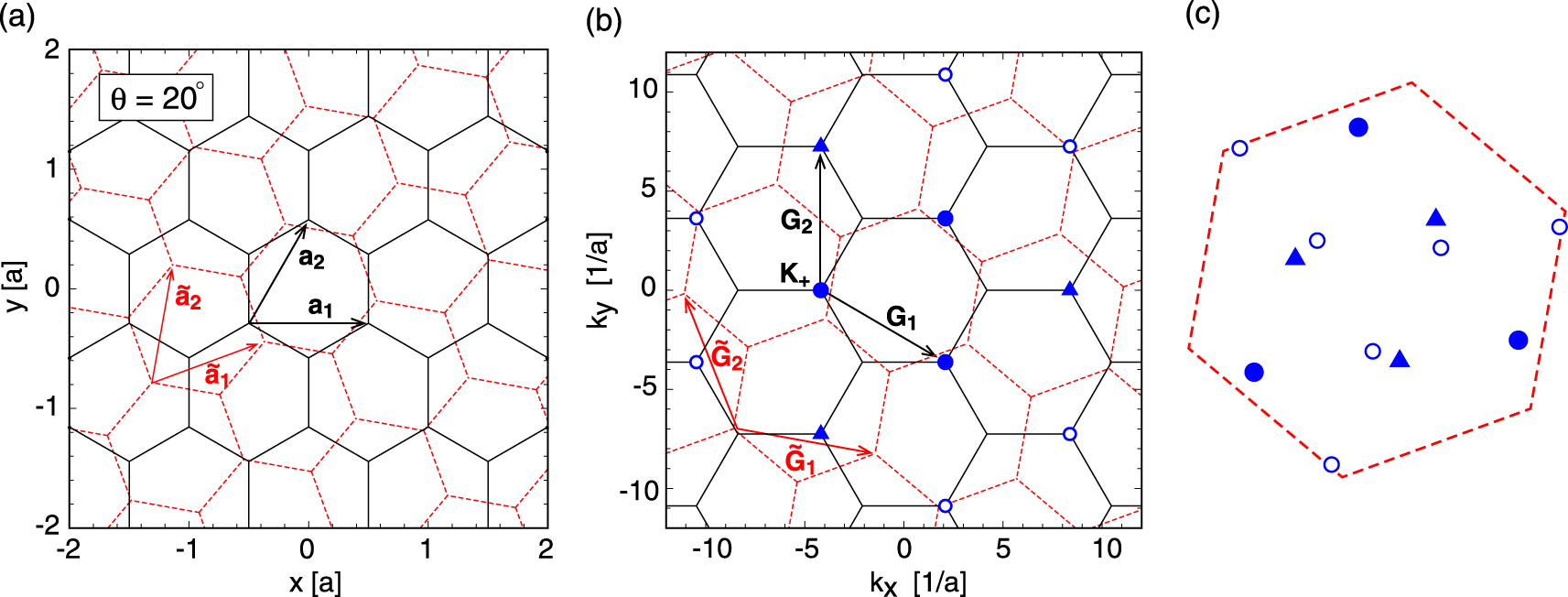
We apply the general formulation obtained above to the irregularly stacked bilayer graphene with an arbitrary rotation angle. Here we consider a pair of hexagonal lattices as shown in figure 2(a), which are stacked with a relative rotation angle θ and interlayer spacing d. We define the primitive lattice vectors of layer 1 as ${{{\bf a}}_{1}}=a(1,0)$ and ${{{\bf a}}_{2}}=a(1/2,\sqrt{3}/2)$ with the lattice constant a, and those of the layer 2 as ${{\tilde{{\bf a}}}_{i}}=R{{{\bf a}}_{i}}$ where R is the rotation matrix by θ. Accordingly, the reciprocal lattice vectors of layer 1 (${{{\bf G}}_{1}},{{{\bf G}}_{2}}$) and layer 2 are related by ${{\tilde{{\bf G}}}_{i}}=R\;{{{\bf G}}_{i}}$. The atomic positions are given by

$$\begin{eqnarray}\begin{array}{rcl} {{{\bf R}}_{X}} & = & {{n}_{1}}{{{\bf a}}_{1}}+{{n}_{2}}{{{\bf a}}_{2}}+{{{\boldsymbol{ \tau }} }_{X}}\qquad \qquad \qquad \qquad ({\rm layer}\ 1), \\ {{{\bf R}}_{\tilde{X}}} & = & {{\tilde{n}}_{1}}{{\tilde{{\bf a}}}_{1}}+{{\tilde{n}}_{2}}{{\tilde{{\bf a}}}_{2}}+{{{\boldsymbol{ \tau }} }_{\tilde{X}}}\qquad \qquad \qquad \qquad ({\rm layer}\ 2), \\ \end{array}\end{eqnarray} \tag{ 13 }$$

for $X=A,B$ (layer 1) and $\tilde{X}=\tilde{A},\tilde{B}$ (layer 2), where

$$\begin{eqnarray}\begin{array}{rcl} {{{\boldsymbol{ \tau }} }_{A}} & = & 0, \\ {{{\boldsymbol{ \tau }} }_{B}} & = & -({{{\bf a}}_{1}}+2{{{\bf a}}_{2}})/3, \\ {{{\boldsymbol{ \tau }} }_{\tilde{A}}} & = & d{{{\bf e}}_{z}}+{{{\boldsymbol{ \tau }} }_{0}}, \\ {{{\boldsymbol{ \tau }} }_{\tilde{B}}} & = & d{{{\bf e}}_{z}}+{{{\boldsymbol{ \tau }} }_{0}}-({{\tilde{{\bf a}}}_{1}}+2{{\tilde{{\bf a}}}_{2}})/3. \\ \end{array}\end{eqnarray} \tag{ 14 }$$

Here we take the origin at an A site, and define ${{{\boldsymbol{ \tau }} }_{0}}$ as the relative in-plane translation vector of the layer 2 to layer 1.

Zoom In Zoom Out Reset image size

To describe the electron's motion, we adopt the single-orbital tight-binding model for p_z atomic orbitals. Then ${{T}_{\tilde{X}X}}({\bf R})$ does not depend on indexes $\tilde{X}$ and X, and it is approximately written in terms of the Slater–Koster parametrization as [37],

$$\begin{eqnarray}\begin{array}{rcl} -T({\bf R}) & = & {{V}_{pp\pi }}\left[ 1-{{\left( \frac{{\bf R}\cdot {{{\bf e}}_{z}}}{d} \right)}^{2}} \right]+{{V}_{pp\sigma }}{{\left( \frac{{\bf R}\cdot {{{\bf e}}_{z}}}{d} \right)}^{2}}, \\ {{V}_{pp\pi }} & = & V_{pp\pi }^{0}{{{\rm e}}^{-(R-a/\sqrt{3})/{{r}_{0}}}},\quad {{V}_{pp\sigma }}=V_{pp\sigma }^{0}{{{\rm e}}^{-(R-d)/{{r}_{0}}}}. \\ \end{array}\end{eqnarray} \tag{ 15 }$$

The typical parameters for graphene are $a\approx 0.246$ nm, $d\approx 0.335\;{\rm nm}$, $V_{pp\pi }^{0}\approx -2.7\;{\rm eV}$, $V_{pp\sigma }^{0}\approx 0.48\;{\rm eV}$, and ${{r}_{0}}\approx 0.184a$ [11]. Once the transfer integral $T({\bf R})$ between the atomic sites is given, one can calculate the in-plane Fourier transform $t({\bf q})$, and then obtain the interlayer Hamiltonian by equation (5). Since the transfer integral is isotropic along the in-plane direction, we can write $t({\bf q})=t(q)$ with $q=\mid {\bf q}\mid$.

Figure 2(a) illustrates the lattice structure at rotation angle θ = 20°. Figure 2(b) shows the Brillouin zones of the two layers in the extended zone scheme, where the blue symbols (filled circles, triangles and open circles) represent the positions of ${\bf k}+{\bf G}$ for some particular ${\bf k}$ (here chosen as the zone corner ${{{\bf K}}_{+}}$) with several ${\bf G}$'s. Figure 2(c) plots the corresponding positions of these symbols inside the first Brillouin zone of layer 2. This indicates the wave numbers of layer 2, $\tilde{{\bf k}}={\bf k}+{\bf G}-\tilde{{\bf G}}$, which are coupled to ${\bf k}$ of layer 1 under the condition of equation (1). The amplitude of the coupling is given by $t({\bf k}+{\bf G})$, and it solely depends on the distance to each symbol from the k-space origin in figure 2(b). In the present parameter choice, the amplitudes for filled circles, triangles and open circles are $t(K)\approx 110$ meV, $t(2K)\approx 1.6$ meV, and $t(\sqrt{7}K)\approx 0.062$ meV respectively, where $K=\mid {{{\bf K}}_{+}}\mid =4\pi /(3a)$. The couplings for other k-points are exponentially small and negligible.

When the lattice vectors of the two layers are incommensurate (i.e., do not have a common multiple) as in this example, we cannot define the common Brillouin zone nor calculate the exact band structure, since the interlayer interaction connects infinite number of k-points in the Brillouin zones of layers 1 and 2. But still, we can obtain an approximate band structure, considering only the first-order interlayer processes while neglecting multiple processes. Let us consider a particular wave vector ${\bf k}$ of layer 1, and take all $\tilde{{\bf k}}$'s in layer 2 which are directly coupled to ${\bf k}$ as in figure 2(c). By neglecting exponentially small matrix elements, we can construct a finite Hamiltonian matrix including only the bases of a single wave vector ${\bf k}$ of layer 1 and several $\tilde{{\bf k}}$'s in layer 2. By diagonalizing the matrix, we obtain the energy eigenvalues ${{\varepsilon }_{n{\bf k}}}$ labeled by the index n. We then define the spectral function contributed from layer 1 as

$$\begin{eqnarray}&&{{A}_{1}}({\bf k},\varepsilon )=\mathop{\sum }\limits_{n}g_{n{\bf k}}^{(1)}\delta (\varepsilon -{{\varepsilon }_{n{\bf k}}}),\end{eqnarray} \tag{ 16 }$$

where $g_{n{\bf k}}^{(1)}$ is the total wave amplitudes on layer 1 in the state $\mid n{\bf k}\rangle$. The density of states contributed from layer 1 is expressed as

$$\begin{eqnarray}&&{{D}_{1}}(\varepsilon )=\mathop{\sum }\limits_{{\bf k}}{{A}_{1}}({\bf k},\varepsilon ),\end{eqnarray} \tag{ 17 }$$

where the summation is taken over the first Brillouin zone of layer 1. We perform the exactly same procedure for the layer 2 by considering a single $\tilde{{\bf k}}$ of layer 2 and all ${\bf k}$'s in layer 1 coupled to $\tilde{{\bf k}}$, and obtain the spectral function and the density of states for the layer 2. The total density of states of the system is given by ${{D}_{1}}+{{D}_{2}}$.

Figure 3 plots the total density of state $D(\varepsilon )$ calculated for the incommensurate bilayer graphene with $\theta =20^{\bf\dot{}}$. The red dashed curve is the density of states of decoupled bilayer graphene (i.e., twice of monolayer's). We actually see additional peak structures due to the interlayer interaction, and these features are consistent with the exact tight-binding calculation for a commensurate bilayer graphene at a similar rotation angle [11]. Figure 4 illustrates the Fermi surface reconstruction at several different energies. The right panel in each row shows the layer 1's spectral function ${{A}_{1}}({\bf k},\varepsilon )$ in presence of the interlayer coupling. The left panel shows the Fermi surface in absence of the interlayer coupling, where the black curves represent the equienergy lines for the layer 1's energy dispersion ${{\varepsilon }_{1}}({\bf k})$, and the pink curves are for the layer 2's dispersion with k-space shift, ${{\varepsilon }_{2}}({\bf k}+{\bf G})$. Thickness of the pink curves indicates the absolute value of the interlayer coupling $t({\bf k}+{\bf G})$.

Zoom In Zoom Out Reset image size

Zoom In Zoom Out Reset image size

Figure 4(a) shows a typical case ($\varepsilon =2.5$ eV) where we observe small band anticrossing at the intersection of the Fermi surfaces of layers 1 and 2. Figure 4(b) ($\varepsilon =-2.85$ eV) is for the energy at which the density of states exhibits a dip (figure 3). There the interlayer coupling is relatively strong, and indeed we see that the original triangular Fermi pockets of the individual layers are strongly mixed and reconstructed into a large single Fermi surface. Note that the coupling strength depends not only on $t({\bf k}+{\bf G})$, but also on the relative phase factors between different sublattices. At even lower energy $\varepsilon =-5$ eV (figure 4(b)) beyond the van-Hove singularity, the layer 1 and the layer 2 have almost identical Fermi surface surrounding Γ point in absence of the interlayer coupling, and they are hybridized into a pair of circles with different radii corresponding to the bonding and anti-bonding states. This feature is also observed in the density of states (figure 3) as a large split of the band bottom. Such a splitting does not occur in the positive energy region, because there A and B sublattices in the same layer have the opposite signs in the wave amplitude, so that the interlayer mixing vanishes due to the phase cancellation.

In the above approximation, we neglect the second order processes such that $\tilde{{\bf k}}$ points of layer 2 (linked from initial ${\bf k}$ of layer 1) are further coupled to other ${\bf k}^{\prime}$ of layer 1. We can include such higher-order processes up to any desired order as follows. To include the second order process in calculating ${{A}_{1}}({\bf k},\varepsilon )$, for example, we take all $\tilde{{\bf k}}$ of layer 2 which are coupled to ${\bf k}$ of layer 1 and also take all ${\bf k}^{\prime}$ of layer 1 which are coupled to $\tilde{{\bf k}}$, and then construct a Hamiltonian matrix with a larger dimension. From the obtained eigenstates, we calculate the spectral function using equation (16), but then $g_{n{\bf k}}^{(1)}$ should be the total wave amplitudes from layer 1 at the original ${\bf k}$ (0-th order), without including ${\bf k}^{\prime}$.

When the primitive lattice vectors of layer 1 and those of layer 2 are slightly different, the interference of two lattice structures gives rise to a long-period moiré pattern, and then we can use the long-range effective theory to describe the interlayer interaction [2–14]. Here we show that the long-range effective theory can be naturally derived from the present general formulation, just by assuming that the two lattice structures are close to each other.

We define a linear transformation with a matrix A that relates the primitive lattice vectors of layers 1 and 2 as

$$\begin{eqnarray}&&{{\tilde{{\bf a}}}_{i}}=A\;{{{\bf a}}_{i}}.\end{eqnarray} \tag{ 18 }$$

Correspondingly, the reciprocal lattice vectors become

$$\begin{eqnarray}&&{{\tilde{{\bf G}}}_{i}}={{({{A}^{\dagger }})}^{-1}}{{{\bf G}}_{i}},\end{eqnarray} \tag{ 19 }$$

to satisfy ${{{\bf a}}_{i}}\cdot {{{\bf G}}_{j}}={{\tilde{{\bf a}}}_{i}}\cdot {{\tilde{{\bf G}}}_{j}}=2\pi {{\delta }_{ij}}$. When the lattice structures of the two layers are similar, the matrix A is close to the unit matrix. The reciprocal lattice vectors of the moiré superlattice are given by small difference between ${{{\bf G}}_{i}}$ and ${{\tilde{{\bf G}}}_{i}}$ as

$$\begin{eqnarray}&&{\bf G}_{i}^{M}={{{\bf G}}_{i}}-{{\tilde{{\bf G}}}_{i}}=[1-{{({{A}^{\dagger }})}^{-1}}]{{{\bf G}}_{i}}.\end{eqnarray} \tag{ 20 }$$

When the two layers are identical and rotationally stacked with a small angle, for example, the matrix A is given by a rotation R. Noting ${{({{R}^{\dagger }})}^{-1}}=R$, we have

$$\begin{eqnarray}&&{\bf G}_{i}^{M}=(1-R){{{\bf G}}_{i}}.\end{eqnarray} \tag{ 21 }$$

When layers 1 and 2 have different lattice constant as in the graphene–hBN bilayer, the matrix A is given by the combination of the isotropic expansion and the rotation as $\alpha R$, where α is the lattice constant ratio. Since ${{[{{(\alpha R)}^{\dagger }}]}^{-1}}={{\alpha }^{-1}}R$, we have

$$\begin{eqnarray}&&{\bf G}_{i}^{M}=[1-{{\alpha }^{-1}}R]{{{\bf G}}_{i}}.\end{eqnarray} \tag{ 22 }$$

When the specific form of the matrix A is given, we can immediately derive the interlayer matrix elements for the long wavelength components using equation (5) as

$$\begin{eqnarray}\begin{array}{rcl} {{U}_{\tilde{X}X}}({\bf k}+{{m}_{1}}{\bf G}_{1}^{M}+{{m}_{2}}{\bf G}_{2}^{M},{\bf k}) & = & -{{t}_{\tilde{X}X}}({\bf k}+{{m}_{1}}{{{\bf G}}_{1}}+{{m}_{2}}{{{\bf G}}_{2}}) \\ {} & {} & \times \;{{{\rm e}}^{-{\rm i}({{m}_{1}}{{{\bf G}}_{1}}+{{m}_{2}}{{{\bf G}}_{2}})\cdot {{\tau }_{X}}+i({{m}_{1}}{{\tilde{{\bf G}}}_{1}}+{{m}_{2}}{{\tilde{{\bf G}}}_{2}})\cdot {{\tau }_{\tilde{X}}}}}, \\ \end{array}\end{eqnarray} \tag{ 23 }$$

where m₁ and m₂ are integers.

For example, let us derive the interlayer Hamiltonian of the irregularly stacked bilayer graphene with a small rotation angle. Since the low-energy spectrum of graphene is dominated by the electronic states around the Brillouin zone corners K and K', we consider the matrix elements for initial and final k-vectors near those points. The K and K' points are located at ${{{\bf K}}_{\xi }}=-\xi (2{{{\bf G}}_{1}}+{{{\bf G}}_{2}})/3$ for layer 1 and ${{\tilde{{\bf K}}}_{\xi }}=-\xi (2{{\tilde{{\bf G}}}_{1}}+{{\tilde{{\bf G}}}_{2}})/3$ for layer 2, where $\xi =\pm 1$ are the valley indexes for K and K', respectively. When we start from ${\bf k}={{{\bf K}}_{+}}$, for example, a typical scattering process is illustrated in figures 5(b) and (c) in a similar manner to figure 2. There the electron at ${{{\bf K}}_{+}}$ in layer 1 is coupled to ${{{\bf K}}_{+}}+{{m}_{1}}{{{\bf G}}_{1}}+{{m}_{2}}{{{\bf G}}_{2}}$ in layer 2 with absolute amplitude $t({{{\bf K}}_{+}}+{{m}_{1}}{{{\bf G}}_{1}}+{{m}_{2}}+{{{\bf G}}_{2}})$. As already argued in the previous section, the coupling amplitudes for filled circles, triangles and open circles in figures 5(b) and (c) are $t(K)\approx 110$ meV, $t(2K)\approx 1.6$ meV, and $t(\sqrt{7}K)\approx 0.062$ meV respectively, and the couplings to other k-points are negligibly small. The matrix element changes when the initial vector ${\bf k}$ is shifted from ${{{\bf K}}_{+}}$, but we neglect such a dependence assuming ${\bf k}$ is close to ${{{\bf K}}_{+}}$. As a result, we obtain the interlayer Hamiltonian of near ${{{\bf K}}_{\xi }}$ from equation (23) as

$$\begin{eqnarray}\begin{array}{rcl} U & = & \left( \begin{array}{ccccccccccccccc} {{U}_{\tilde{A}A}} & {{U}_{\tilde{A}B}} \\ {{U}_{\tilde{B}A}} & {{U}_{\tilde{B}B}} \\ \end{array} \right) \\ {} & = & t(K)\left[ \left( \begin{array}{ccccccccccccccc} 1 & 1 \\ 1 & 1 \\ \end{array} \right)+\left( \begin{array}{ccccccccccccccc} 1 & {{\omega }^{-\xi }} \\ {{\omega }^{\xi }} & 1 \\ \end{array} \right){{{\rm e}}^{{\rm i}\xi {\bf G}_{1}^{{\rm M}}\cdot {\bf r}}}+\left( \begin{array}{ccccccccccccccc} 1 & {{\omega }^{\xi }} \\ {{\omega }^{-\xi }} & 1 \\ \end{array} \right){{{\rm e}}^{{\rm i}\xi ({\bf G}_{1}^{{\rm M}}+{\bf G}_{2}^{{\rm M}})\cdot {\bf r}}} \right] \\ {} & {} & +t(2K)\left[ \left( \begin{array}{ccccccccccccccc} 1 & 1 \\ 1 & 1 \\ \end{array} \right){{{\rm e}}^{{\rm i}\xi (2{\bf G}_{1}^{{\rm M}}+{\bf G}_{2}^{{\rm M}})\cdot {\bf r}}}+\left( \begin{array}{ccccccccccccccc} 1 & {{\omega }^{-\xi }} \\ {{\omega }^{\xi }} & 1 \\ \end{array} \right){{{\rm e}}^{{\rm i}\xi {\bf G}_{2}^{{\rm M}}\cdot {\bf r}}}+\left( \begin{array}{ccccccccccccccc} 1 & {{\omega }^{\xi }} \\ {{\omega }^{-\xi }} & 1 \\ \end{array} \right){{{\rm e}}^{-{\rm i}\xi {\bf G}_{2}^{{\rm M}}\cdot {\bf r}}} \right] \\ {} & {} & +\cdots , \\ \end{array}\end{eqnarray} \tag{ 24 }$$

where ${\bf r}$ is the in-plane position, $\omega ={\rm exp} (2\pi {\rm i}/3)$ and ${{{\boldsymbol{ \tau }} }_{0}}$ is set to 0.

Zoom In Zoom Out Reset image size

The total Hamiltonian is written in the basis of $\{A,B,\tilde{A},\tilde{B}\}$ as

$$\begin{eqnarray}U_{{\rm eff}}^{(\xi )}=\left( \begin{array}{ccccccccccccccc} {{H}_{1}} & {{U}^{\dagger }} \\ U & {{H}_{2}} \\ \end{array} \right),\end{eqnarray} \tag{ 25 }$$

where H₁ and H₂ are the intralayer Hamiltonian of layers 1 and 2, respectively, defined by

$$\begin{eqnarray}\begin{array}{rcl} {{H}_{1}} & \approx & -\hbar v({\bf k}-{{{\bf K}}_{\xi }})\cdot (\xi {{\sigma }_{x}},{{\sigma }_{y}}), \\ {{H}_{2}} & \approx & -\hbar v[{{R}^{-1}}({\bf k}-{{\tilde{{\bf K}}}_{\xi }})]\cdot (\xi {{\sigma }_{x}},{{\sigma }_{y}}), \\ \end{array}\end{eqnarray} \tag{ 26 }$$

with Pauli matrices ${{\sigma }_{x}}$ and ${{\sigma }_{y}}$, and the graphene's band velocity v. If we only take the terms with t(K) in the matrix U, the expression becomes consistent with the previous formulation for graphene–graphene bilayer [2, 7, 8, 11]. Note that the Hamiltonian matrix depends on the actual choice of K points out of the equivalent Brillouin zone corners; ${{{\bf K}}_{\xi }}+{{m}_{1}}{{{\bf G}}_{1}}+{{m}_{2}}{{{\bf G}}_{2}}$ and ${{\tilde{{\bf K}}}_{\xi }}+{{\tilde{m}}_{1}}{{\tilde{{\bf G}}}_{1}}+{{\tilde{m}}_{2}}{{\tilde{{\bf G}}}_{2}}$. The different choice of m_i and ${{\tilde{m}}_{i}}$ adds extra phase factors to the Bloch bases depending on sublattices, while the resulting Hamiltonian matrix are connected to the original by an unitary transformation.

While we neglected the interlayer translation vector ${{{\boldsymbol{ \tau }} }_{0}}$ in deriving equation (24), the matrix elements of U actually depend on ${{{\boldsymbol{ \tau }} }_{0}}$ according to equation (23), where the term with ${{{\rm e}}^{{\rm i}({{m}_{1}}{\bf G}_{1}^{{\rm M}}+{{m}_{2}}{\bf G}_{2}^{{\rm M}})\cdot {\bf r}}}$ is accompanied by an additional phase factor ${{{\rm e}}^{{\rm i}({{m}_{1}}{{\tilde{{\bf G}}}_{1}}+{{m}_{2}}{{\tilde{{\bf G}}}_{2}})\cdot {{\tau }_{0}}}}$. This extra term, however, can be incorporated into a shift of the space origin as

$$\begin{eqnarray}&&{{{\rm e}}^{{\rm i}({{m}_{1}}{\bf G}_{1}^{{\rm M}}+{{m}_{2}}{\bf G}_{2}^{{\rm M}})\cdot {\bf r}}}\;{{{\rm e}}^{{\rm i}({{m}_{1}}{{\tilde{{\bf G}}}_{1}}+{{m}_{2}}{{\tilde{{\bf G}}}_{2}})\cdot {{\tau }_{0}}}}={{{\rm e}}^{{\rm i}({{m}_{1}}{\bf G}_{1}^{{\rm M}}+{{m}_{2}}{\bf G}_{2}^{{\rm M}})\cdot ({\bf r}+{{{\bf r}}_{0}})}},\end{eqnarray} \tag{ 27 }$$

where

$$\begin{eqnarray}&&{{{\bf r}}_{0}}=(A-1){{{\boldsymbol{ \tau }} }_{0}}.\end{eqnarray} \tag{ 28 }$$

This reflects the fact that relative sliding between two layers leads to a shift of the moiré interference pattern in the real space. The only exception is when the two layers share the same lattice vectors ${{{\bf G}}_{i}}={{\tilde{{\bf G}}}_{i}}$, where ${\bf G}_{i}^{{\rm M}}$ vanishes so that ${{{\boldsymbol{ \tau }} }_{0}}$ cannot be eliminated by shifting the origin. In this case, the energy band actually becomes different depending on the sliding vector ${{{\boldsymbol{ \tau }} }_{0}}$. For the graphene bilayer case, in particular, the expression of U with ${{{\bf G}}_{i}}={{\tilde{{\bf G}}}_{i}}$ becomes equivalent to that of regularly-stacked graphene bilayer with an interlayer sliding [38–40].

We theoretically studied the interlayer interaction in general incommensurate bilayer systems with arbitrary crystal structures. By using the generic tight-binding description, we demonstrate that the interlayer coupling in the reciprocal space is simply expressed in terms of a generalized Umklapp process. We applied the formulation to the incommensurate honeycomb lattice bilayer with a large rotation angle, which cannot be treated as a long-range moiré superlattice, and actually obtain the quasi band structure and density of states within the first-order approximation. Finally, we apply the formulation to the moiré superlattice where the two lattice structures are close, and derive the long-range effective theory with a straightforward calculation.

This work was supported by JSPS Grant-in-Aid for Scientific Research No. 24740193 and No. 25107005.