


Abstract
Single-photon-level non-Gaussian operations—photon addition, photon subtraction, and their coherent superposition—are powerful tools with which to increase entanglement in continuous-variable optical states. Although such operations are typically not deterministic, there may be other advantages such as noiseless manipulation. Therefore, to fully account for the efficacy of a particular non-Gaussian operation in a practical scenario, we develop figures of merit which trade off the advantages of such protocols against their success probability. Specifically, we define 'entanglement enhancement rate' as the increase in entanglement per trial of a generic non-Gaussian operation on a two-mode squeezed vacuum (TMSV) state. We consider states generated by photon-subtraction, photon-addition and a coherent superposition of subtraction and addition. We compare each strategy when applied to one or both modes of a TMSV state, and also in the presence of channel losses prior to the operation. In many cases, additional properties are analytically calculable, including excess noise arising from the operation and the fidelity of the resulting states to particular Gaussian and non-Gaussian states. Finally, by incorporating loss, we derive optimal interaction parameters for each non-Gaussian operation which maximize the effectiveness of the particular protocol under investigation.
Export citation and abstract BibTeX RIS

Content from this work may be used under the terms of the Creative Commons Attribution 3.0 licence. Any further distribution of this work must maintain attribution to the author(s) and the title of the work, journal citation and DOI.
1. Introduction
Entanglement is an important resource upon which many quantum communication protocols are based. However, it is a fragile resource susceptible to decoherence—in an optical setting this is mainly induced by loss. Therefore, the ability to increase the amount of entanglement available is a useful strategy to overcome that which may be lost during transmission. In the continuous-variable (CV) domain, one important entangled resource state is the two-mode squeezed vacuum (TMSV), a state which may be created deterministically by nonlinear optical processes. The TMSV is an example of a Gaussian state, whereby the first and second moments of its Wigner function uniquely describe the state. Although such states can be generated on-demand, Gaussian states require at least one non-Gaussian state and/or operation in order to increase their entanglement [1]. Since the nonlinearities necessary for non-Gaussian operations—at least 3rd order—are so small at the single-photon level, such nonlinearities must normally be induced by measurement [2].
Single-photon-level non-Gaussian operations such as photon subtraction [3–15], photon addition [4, 12, 16, 17] and a coherent superposition of addition and subtraction [18–20], here termed photon replacement, are powerful tools which, under certain conditions, can be used to increase entanglement. In the case of photon subtraction, the entanglement-enhancing capability has been experimentally demonstrated [21–23].
In all cases, there is a fundamental trade-off between success probability of each operation and the resultant increase in entanglement. In addition to investigating the increase in entanglement, previous analyses of these processes have adopted different figures of merit to compare each protocol, for example teleportation fidelity [3–5, 9, 10], log-negativity [6, 8, 11, 14, 17, 20] or entanglement entropy [12, 19]. However, the probabilistic nature of these operations, and the implications thereof, have been largely overlooked. Indeed, in the case of both subtraction and addition, we will show that these figures of merit are maximized when the probability of a successful event is precisely zero. By contrast, the photon replacement operation maximizes entanglement at non zero probability. However, photon replacement, and indeed photon addition, requires additional ancillary photons, the production of which is not deterministic. Strictly speaking, one must also account for the probability associated with the production of photons when considering the probability of a success of the protocol.
Furthermore, analyses up to now consider that failure modes can be freely discarded without consequence. This may not be the case for all protocols; the corollary of accounting for success must therefore be to properly account for the failure modes and any negative effects these may have on the protocol.
A number of factors influence the efficacy of practical entanglement enhancement protocols. One might be interested in, for example:
- the total entanglement generated;
- the probability of success of a protocol;
- the rate at which entanglement is increased;
- the 'quality' of the states generated, i.e. their suitability for a particular task, e.g. teleportation fidelity [24];
- the resource costs of running each protocol;
- the tolerance of loss.
If entanglement-based quantum communication is to become widespread, at least some of such factors should be considered collectively and, where possible, quantified.
In this paper, we investigate the probabilities associated with photon subtraction, photon addition and photon replacement (the coherent superposition of subtraction and addition) on a TMSV state, in order to provide a practical comparison between them. In section 2 we will briefly review each operation . In section 3, we will define figures of merit accounting for the success probabilities with which each operation can be compared. We also calculate further figures of merit which include a measure of Gaussianity based on the quantum relative entropy (QRE) [25, 26] induced by the non-Gaussian operation, as well as fidelity to certain Gaussian and non-Gaussian states. In section 4 we will include an analysis of loss in each case. Finally, we will conclude in section 5.
2. Non-Gaussian operations
The starting point for all operations is the two-mode squeezed state

which is characterized by the squeezing parameter λ. The normalized coefficients of the Schmidt decomposition, cn, are the probability amplitudes of the state existing in the state  . These cn may be modified by partial measurement of the state.
Our metric of the entanglement contained in such a state is the log-negativity En, the logarithm of the sum of the negative eigenvalues of the partially transposed density matrix [27]. For pure states written in the Schmidt form, i.e.  , it is given by

where cn are the normalized Schmidt coefficients. Thus a TMSV has entanglement  , which is the benchmark from which all changes in entanglement resulting from the non-Gaussian operations will be measured. In the remainder of this section, we will review each operation and the form and properties of the resulting non-Gaussian states.
A schematic for all the operations is shown in figure 1, whereby each case is governed by different ancilla Fock states  and perfect photon-number projective measurements
  .
.

Figure 1. Setup for performing measurement-induced nonlinear operations on a two-mode squeezed state. Each mode of a TMSV  undergoes interference at a beam splitter of transmissivity
  with an ancilla mode
  , followed by projective photon-number measurement
  . This conditional interaction results in the final state
  .
.
Download figure:
Standard image High-resolution imageThe key parameter in each of these processes—one which is under direct control of the experimentalist—is the beam splitter transmissivity  . The value of
  not only dictates the resulting state
  but also the probability of the desired projective measurement outcome.
2.1. Photon subtraction
Photon subtraction [3, 4] is perhaps the most straightforward non-Gaussian conditional operation to carry out [7, 28].
In symmetric photon subtraction, we consider the case where one photon is subtracted from each mode; that is,  and
and  in figure 1. The resulting state is
where  is the reflectivity of the subtracting beam splitters and
  is a normalization constant. Writing
  in this form relates this constant to the probability of subtracting a photon
  , i.e.

The log-negativity of this state, calculated following equation (2), is given by

For a particular range of T and λ, the log-negativity is greater than that of the initial TMSV, as we will show in section 3. Increasing entanglement by photon subtraction has been experimentally demonstrated [22, 23].
2.1.1. Single-mode photon subtraction
In asymmetric photon subtraction, we consider the case in which photons are subtracted from one mode only, and the other mode is left unimpeded. In this case, the ancilla states remain  , as does one of the projective measurements, e.g.
  as in the two-mode case; but no subtraction occurs on the other mode, i.e.
  and
and  .
.
The state that results following this operation is

where T is the transmissivity of the beam splitter in subtracted mode. This event has a probability  given by

The state given in equation (5), although pure, is not of the form  , therefore we cannot use equation (2) to derive an analytic form for the log-negativity of the state. However, we have previously shown how an exact form for the log-negativity can be found [14]. In the results that follow, the log-negativity was calculated numerically.
2.2. Photon addition
Symmetric photon addition consists of single photons in the ancilla modes  and vacuum projection
  in the detected mode. This creates the state

where again  is the transmissivity of both beam splitters in figure 1 and
  is the probability of photon addition, given explicitly by

For fixed transmissivity T, this is always greater than  by a factor of
  .
.
The log-negativity of this state  is identical to the subtracted case:

Again, for a range of  , entanglement may be increased from the initial value.
2.2.1. Single-mode photon addition
Similarly, asymmetric photon addition comprises a single ancilla photon added to just one mode, e.g.  ,
,  and
and  . This operation creates the state

with probability

Again, this probability is a factor of  greater than single-mode photon subtraction.
Regarding the experimental feasibility of photon addition, it is immediately apparent that it is more involved than subtraction. In the model described above, one requires a reservoir of single photons to add to the correct mode, and vacuum detection to herald success. Despite considerable effort, on-demand single-photon sources—particularly sources of photons mode-matched to squeezed states—have not yet been demonstrated . Furthermore, vacuum projection onto the correct mode is experimentally challenging, and is also yet to be shown experimentally. This is largely because extremely high-efficiency detectors are required, although such detectors [29] are beginning to be used [30, 31]. To overcome both of these problems, experimental schemes typically use seeded parametric down-conversion to herald photons added to the mode of interest [32–35]. This approach requires a much more detailed model of the nonlinear interaction producing the added photons, which is beyond the scope of the present work.
2.3. Photon replacement
Photon replacement [18, 19] is a coherent superposition of the subtraction and addition operations, leaving the same total number of photons in the beam after the operation as before it. In a state engineering context, this operation has also been termed 'quantum catalysis' [36, 37]. A photon-replaced state is generated by interfering a mode with a single-photon ancilla state, and projecting one output of the interference onto a single-photon state. In general, acting on a single mode, the photon replacement operation enacts the operation [38]

where  is a normalization constant depending on T.
In figure 1, single-mode replacement, rep(1), corresponds to  , while two-mode replacement, rep(2), shown explicitly in figure 2, corresponds to
  .
.
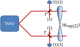
Figure 2. Setup for two-mode photon replacement. The success probabilities  for these operations and the final entanglement
  depend on the beam splitter transmissivity
  .
.
Download figure:
Standard image High-resolution imageUnlike photon subtraction and addition, this operation conserves photon number in the resultant mode, leading to some interesting features. For example, one replacement operation on each mode (two-mode photon replacement) for which the transmissivities of the beam splitters are equal, is entirely equivalent to two iterations of single photon replacement on the same mode, as can be seen from equation (12)1 . The one- and two-mode photon-replaced states, rep(1) and rep(2) are given by


and the probability of the conditioning measurement in each case is


Unlike the single-mode subtracted and added states, the log-negativity of the single-mode replaced state is analytically tractable, since it is of the form required for equation (2) (i.e. it remains a number-correlated state). For the single-mode replaced state  , given
  , the only positive cn is c0. All other
  are negative for the range
  . On the other hand, calculating the entanglement in the case where photons are replaced in both modes
  requires no such manipulation since the Schmidt coefficients are always positive. For each case, the entanglement is given by
whereby the expression for  is valid for
  .
.
3. Figures of merit
Equipped with the expressions for the entanglement and success probabilities of each of the entanglement-enhancing non-Gaussian operations, we are now in a position to compare and contrast them in an operational sense. Based on the considerations of a realistic entanglement-enhancement protocol above, any number of figures of merit can be constructed. We suggest several and show how each entanglement-enhancing non-Gaussian operation performs.
3.1. Total entanglement
Perhaps the most straightforward question to ask is how much entanglement exists after a successful measurement-induce non-Gaussian operation. This is shown in figure 3; as a function of beam splitter transmissivity T and initial squeezing λ, the total entanglement resulting from single- and two-mode operations are shown in figures 3(a) and (b), respectively. It is apparent from figure 3(c)—a cross-section of figures 3(a) and (b) at  —that photon replacement, both from one and two modes, produces more entanglement than subtraction/addition at low initial squeezing, the most experimentally accessible region. For subtraction and addition, the entanglement dependence on these parameters are equal, and approach the maximum value as
  for all λ. The replacement schemes have maxima that depend on λ: at
  these occur at T = 0.1 and T = 0.27 for single- and double-photon replacement, respectively.

Figure 3. Log-negativity as a function of interaction parameters T (beam splitter transmissivity) and λ (initial squeezing) for (a) single-mode non-Gaussian operations and (b) two-mode operations. The initial entanglement is shown in semi-transparent grey in both plots. (c): A cross-section through (a) and (b) at  .
.
Download figure:
Standard image High-resolution image3.2. Success probability
As with all nondeterministic operations, success probability is an important quantity. In figure 4 we show the probability for each scheme as a function of the initial squeezing λ and beam splitter transmissivity T.

Figure 4. Success probability of (a) single-mode non-Gaussian operations and (b) two-mode operations . (c) Probability as a function of beam splitter transmissivity T at  .
.
Download figure:
Standard image High-resolution imageIt is clear that protocols that involve introducing an extra photon are more probable; all but photon subtraction have probabilities greater than 10−2 for some set of parameters. However, this requires a source of single-photon ancilla states that are readily accessible.
3.2.1. Probability of ancilla photon generation
While a range of technologies exist which generate single photons [39], true on-demand single-photon states are not yet available. Furthermore, for the schemes described above to be successful, photons from the TMSV state must be indistinguishable from the ancilla photons taking part in the operation (i.e. photons added or replaced). One approach is to use heralded single-photon generation from an identical source of TMSV states. In this case, the probability of generating a heralded single photon is  . It is therefore reasonable to incorporate this probability in the success probability of each protocol when considering their practical application.
In the case of single photon replacement on one mode of a TMSV, an additional factor  is required. For double replacement, two photons are required, therefore the additional factor is
  . The same is true for photon addition on both modes.
It is interesting to note from figure 4 that the probability of single-mode addition, with the probability of ancilla photon generation included, is identical to the probability of single-mode photon subtraction. In turn, this probability is of similar magnitude to single-mode replacement, indicating some level of 'conservation of difficulty'.
3.3. Combining entanglement and probability
To consider the effects of both final entanglement and success probability, we can use the beam splitter transmissivity T to parametrically plot these quantities as a function of initial squeezing λ. This is shown in figure 5. Figures 5(a) and (b) show that subtraction and addition out-perform replacement as the initial squeezing increases. However, at low squeezing, the replacement operations are optimal. This is particularly clear from figure 5(c): for initial squeezing  , single-mode replacement produces the most entanglement at the highest probability. Note also that in this particular figure of merit, photon subtraction never outperforms photon addition.

Figure 5. Parametric plot of final entanglement and success probability of (a) single-mode and (c) two-mode non-Gaussian operations and (c) as above taking  .
.
Download figure:
Standard image High-resolution image3.3.1. Entanglement rate
Perhaps most interesting from figures 3 and 4 is that the replacement schemes produce the highest entanglement at reasonable probabilities. In subtraction and addition, the highest increase in entanglement occurs when T = 1, for which the probability is precisely zero. However, the optimal transmissivities for single and double replacement are, for  , T = 0.1 and T = 0.27 respectively, corresponding to success probabilities 0.02 and 0.01, respectively.
To account for this property, we can define a new figure of merit, the entanglement rate  , by simply multiplying entanglement and probability together, that is

where  are the initial and final states, respectively. This gives the average entanglement per trial of the protocol, and is shown for the four protocols in figure 6. Here again, it is clear that protocols that introduce a single photon give a higher entanglement rate.

Figure 6. Entanglement per trial of a non-Gaussian operation: (a) single-mode operations; (b) two-mode photon operations; (c) entanglement per trial given initial squeezing  .
.
Download figure:
Standard image High-resolution image3.3.2. Entanglement difference
In addition to the absolute level of entanglement obtained following a successful protocol, and the rate at which this is achieved, one may also be interested in the absolute increase in entanglement. We define this as the entanglement difference,  , which is calculated

and shown in figure 7. Again, this plot confirms that at experimentally accessible values of initial squeezing λ, both single- and double-mode photon replacement yields the highest increase in entanglement.
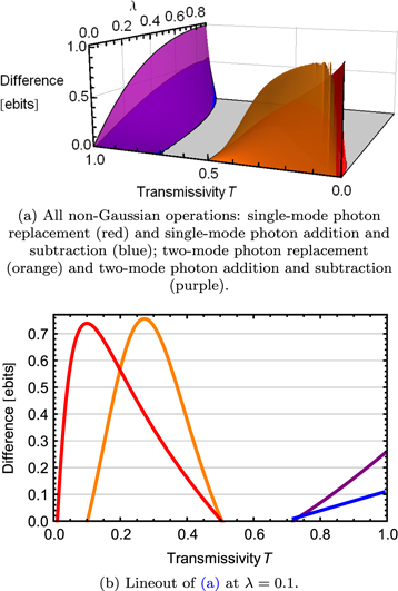
Figure 7. Entanglement difference following each non-Gaussian operation. (a) Difference as a function of interaction parameters beam splitter transmissivity T and initial squeezing λ; (b) difference as a function of T at  . Note that this 2D line-out corresponds directly to figure 3(c).
Download figure:
Standard image High-resolution image3.3.3. Enhancement rate
From the expression for the entanglement difference, we can calculate the average increase per trial, which we define as the enhancement rate  , where

As it is a difference in log-negativities multiplied by a probability (necessarily dimensionless), this has units of ebits. This is shown in figure 8. Again, this confirms that single-mode photon replacement performs better than the other protocols.

Figure 8. Enhancement rate (increase in entanglement increase per trial) of a non-Gaussian operation. (a) Rate as a function of initial squeezing λ and beam splitter transmissivity T; (c) rate given initial squeezing  .
.
Download figure:
Standard image High-resolution imageBy accounting for success probability, the enhancement rate is a clear operational measure of the efficacy of an entanglement-enhancing non-Gaussian operation. Figure 8 clearly shows that there exists an optimal transmissivity T—an experimentally tunable parameter—which maximizes this quantity. This is shown in figure 9(a), as a function of initial squeezing λ.
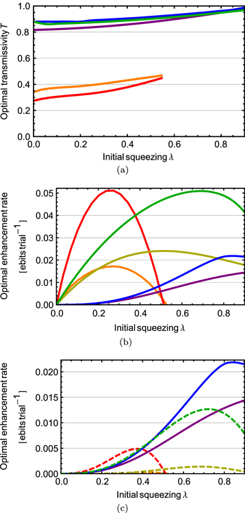
Figure 9. (a) Optimal beam splitter transmissivity T for an initial squeezing λ which maximizes the entanglement enhancement rate for different non-Gaussian operations. Note that  for two-mode subtraction and addition are equal. The resulting enhancement rate at the optimal transmissivity: (b) assuming on-demand ancilla state generation and (c) incorporating probabilistic photon sources (dotted lines indicate changes from (b)).
Download figure:
Standard image High-resolution imageWhen comparing the different strategies, it is sensible to compare each at its optimal set of controllable parameters. Therefore, having extracted the optimal T in order to maximize enhancement rate—i.e. the T which produces the highest increase in entanglement most often—we can plot the resulting optimal enhancement rate as a function of initial squeezing. This is shown in figure 9(b). It is clear that different strategies are best in different regimes of squeezing: single-mode photon replacement is best for  , whereas single-mode photon addition is best for
  . Note that neither replacement operation increases entanglement for
  .
.
This analysis presumes on-demand generation of the necessary ancilla photons for each operation. However, when we include the probability of generating these single photons, the situation changes, as shown in figure 9(c). Single-mode photon replacement is still optimal at initial squeezing below  , after which single-mode subtraction or addition becomes optimal.
3.4. Utility
In terms of log-negativity, all entangled states are equal, but some are more equal than others. That is to say, our states have more entanglement than the two-mode squeezed state with which we started (at least for some range of parameters), but are they any more useful? Utility in this sense depends entirely on the protocol to be employed. To that end, we investigate a number of figures of merit relating to tasks that require entanglement and calculate them for the four states. To obtain anlytic results, we include only those non-Gaussian operations which generate photon-number correlated states, i.e. those states of the form  (single-mode subtraction and addition are omitted).
3.4.1. Gaussianity
One of the principal motivations behind CV entanglement distillation is to generate Gaussian states with higher entanglement than the initial two-mode squeezed states. To quantify the Gaussianity of our state, we use the QRE proposed in [25] (see also [26, 40]). This is defined as the difference in entropy between the state of interest ρ and the closest Gaussian state  —that is, a state fully described by the same mean and covariance matrix.
The QRE  of a general state ρ is calculated by

where ![$S\left( \varrho \right)={\rm Tr}\left[ \varrho {\rm log} \left( \varrho \right) \right]$](https://content.cld.iop.org/journals/1367-2630/17/2/023038/revision1/njp508735ieqn77.gif) is the von Neumann entropy of the state ϱ. Note that for pure states, the von Neumann entropy is zero, therefore the QRE is given by
is the von Neumann entropy of the state ϱ. Note that for pure states, the von Neumann entropy is zero, therefore the QRE is given by  . Using the method outlined in [26], we find that the QRE for two-mode number-correlated pure states of the form
  is
is

where  and expressions for
  and
and  for each state are given in appendix
The QRE for each state is plotted in figure 10. This shows that subtraction returns the state closest to a Gaussian state, whereas the photon-added state is highly non-Gaussian, exhibiting significant QRE. The QRE produced by the photon replacement schemes depends strongly on the parameters.

Figure 10. Quantum relative entropy (QRE) following the non-Gaussian operation. This measures the level of non-Gaussianity for states following different non-Gaussian operations. (a) QRE as a function of initial squeezing λ and beam splitter transmissivity T; (b) QRE given initial squeezing  .
.
Download figure:
Standard image High-resolution image3.4.2. Gaussian state overlap: TMSV
Related to the Gaussianity of the state is its fidelity to a two-mode squeezed state of equivalent entanglement. That is, given a state with entanglement EN, what is its fidelity to a TMSV exhibiting the same log-negativity. We therefore define an effective squeezing parameter  , which is the squeezing parameter of the TMSV with the same entanglement as the non-Gaussian state. This is calculated by

such that the fidelity between the non-Gaussian state  and the effective TMSV
  is readily calculated

where cn are the normalized Schmidt coefficients of the non-Gaussian state  . This is shown in figure 11.
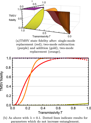
Figure 11. Fidelity to a two-mode squeezed vacuum (TMSV) state of equivalent entanglement following different non-Gaussian operations. (a) Fidelity as a function of initial squeezing λ and beam splitter transmissivity T; (b) fidelity given initial squeezing 
Download figure:
Standard image High-resolution imageThe subtracted state is very close to a TMSV, while the added state exhibits almost no overlap. Both photon-replaced states vary smoothly between low and high overlap in the parameter region corresponding to increasing entanglement from the initial two-mode squeezed state.
A related measure is the 'squeezed vacuum affinity,' introduced in [9]. This metric maximizes the overlap between a non-Gassian state and a TMSV state, with the vacuum squeezing as a free parameter. The two measures are not equivalent: the entanglement of a non-Gaussian state may well differ from the entanglement present in the closest Gaussian state (i.e. the Gaussian state the minimizes the overlap).
3.4.3. Non-Gaussian state overlap: Bell state
Another relevant set of important non-Gaussian entangled states is the set of Bell states. Number-correlated states of the kind in which we are interested can approximate the Bell state

where ϕ is a free parameter. The accuracy of the approximation is given by their overlap  .
.
In this case, as shown in figure 12, neither the subtracted nor added states exhibit significant overlap with the Bell state ( for
for  ). By contrast, the double mode replaced state has 99.95% overlap with a Bell state of phase
  at
at  , while the single-photon replaced state exhibits 99.98% overlap with the bell state of phase
  for T = 0.098 when
  .
.
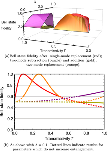
Figure 12. Fidelity to the Bell state  following different non-Gaussian operations. (a) Fidelity as a function of initial squeezing λ and beam splitter transmissivity T; (b) fidelity given initial squeezing
  .
.
Download figure:
Standard image High-resolution imageInterestingly, these are exactly the parameters at which entanglement is maximized, shown in figure 3(c).
3.5. Teleportation
A typical motivation behind distributing entanglement is to facilitate a quantum teleportation protocol [24, 41–45]. Teleportation is a quantum communication task which comprises mapping quantum states from one mode to another, without the modes themselves interacting. The fidelity with which this is achieved is a metric for success of the protocol. Indeed, early theoretical work used the teleportation fidelity as the principal figure of merit for entanglement-enhancement strategies [3–5].
Teleportation fidelities following the non-Gaussian operations described have been compared (independently) by Lee et al [19]. Here, we expand on their results by probing the range of parameters that enhance teleportation for each operation.
3.5.1. Teleportation fidelity
The average teleportation fidelity  can be calculated by [46]

where  is known as the transfer operator,
  is the state to be teleported and the integral is over all phase space. For ancillary entangled states of the form
  , Cochrane et al [4] showed that the transfer operator may be written

where  is a displacement β in phase space given a gain g of the teleporter. For the purposes of this paper, we set g = 1 since we do not consider gain.
When teleporting a coherent state,  , the average fidelity is independent of α. In this case, the expression for average teleportation fidelity
  is
is

For a two-mode squeezed state, the teleportation fidelity is given by

Following each of the non-Gaussian operations, the teleportation fidelities of the resulting states are given by


Note that  is too lengthy to display adequately here; its expression is given in appendix
We plot these fidelities in figure 13. From these plots it is apparent that not all entanglement-enhancing non-Gaussian operations increase the teleportation fidelity. Indeed, there is no region for which photon addition or single-mode photon replacement are better than the original TMSV state in terms of teleportation fidelity, even though they exhibit more entanglement. Therefore, if the purpose of the protocol is to increase teleportation fidelity, then two-mode subtraction or two-mode photon replacement is the only option.

Figure 13. Teleportation fidelity of a coherent state using the two-mode entangled resource state following different non-Gaussian operations. (a) Fidelity as a function of initial squeezing λ and beam splitter transmissivity T; (b) fidelity given initial squeezing  The dotted lines show the region for which entanglement is not increased following the non-Gaussian operation.
Download figure:
Standard image High-resolution image3.5.2. Quantum bounds
Ralph and Lam [43] showed that for teleportation to be unambiguously quantum, the average fidelity must exceed  (see also Grosshans and Grangier [47]). In figure 14, we show where a TMSV, subtracted state and double-mode photon-replaced state exceed this bound as a function of initial squeezing λ. Note that for the subtracted state we have assumed T = 1 (i.e. an operation producing the highest entanglement but with vanishing success probability), and for the photon-replaced state, T is optimized to maximize the fidelity for each λ.

Figure 14. Teleportation fidelity as a function of λ following different non-Gaussian operations: two-mode subtraction (purple) and two-mode replacement (orange). The fidelity of the original TMSV is shown in dashed grey. Fidelities greater than  (blue shaded region) require state reproduction that is unambiguously quantum [43], while fidelities above
  require entanglement during the teleportation protocol [44].
Download figure:
Standard image High-resolution imageThe different states reach the Ralph–Lam bound for different λ: double-mode photon replacement at  (and T = 0.33), photon subtraction at
  and the original TMSV at
  . Therefore, replacement appears to be a good strategy for teleportation at low λ (it is also far more probable in this parameter range, as per figure 4).
3.5.3. Entanglement utility
The final property we will consider is the efficiency with which entanglement in a state is used in a teleportation protocol. That is to say, given a fixed amount of entanglement, which state produces the highest teleportation fidelity? This is shown in figure 15. Both subtraction and double replacement produce states that use entanglement similarly efficiently as a TMSV. However, given the initial squeezing required to generate the final entanglement, in each case, the two-mode replacement operation appears to use the initial entanglement more efficiently.
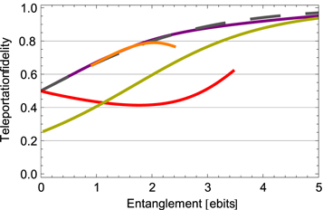
Figure 15. Teleportation fidelity as a function of entanglement following different non-Gaussian operations: single-mode replacement (red); two-mode subtraction (purple) and addition (gold), two-mode replacement (orange).
Download figure:
Standard image High-resolution image4. Loss
We now consider the case where losses in the channel prior to the non-Gaussian operation play a role. The schematic in this case is shown in figure 16, whereby additional beam splitters of transmissivities  introduce loss modes. In the case of photon subtraction, losses at various stages of the protocol can be modelled as a single channel efficiency parameter [14]. While this is not generally true for all non-Gaussian operations, we consider photon losses prior to any non-Gaussian operation as the principle source of loss in a realistic scenario2
.
introduce loss modes. In the case of photon subtraction, losses at various stages of the protocol can be modelled as a single channel efficiency parameter [14]. While this is not generally true for all non-Gaussian operations, we consider photon losses prior to any non-Gaussian operation as the principle source of loss in a realistic scenario2
.
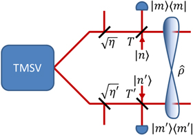
Figure 16. Model of non-Gaussian operations incorporating channel losses  in each mode.
Download figure:
Standard image High-resolution imageWhile allowing different channel efficiencies on each mode is more general (and studied for photon subtraction [14]), we limit ourselves to the case of symmetric loss in each channel, i.e. that  . Furthermore, we do not consider losses at any other point in the protocol, for example in the heralding of the ancilla states required in the addition and replacement operations.
4.1. Entanglement behaviour under loss
In section 3.3.3 we identified enhancement rate  as a useful figure of merit to compare probabilistic entanglement enhancing operations. In the absence of loss, enhancement rate depends on the initial squeezing λ and beam splitter transmissivity T, and we found the optimal T which maximized
  for a given λ.
When accounting for loss, we can again find the optimal transmissivity which maximizes  for a given initial squeezing λ and channel efficiency η. This, along with the enhancement rate it generates, is shown in figure 17.

Figure 17. (a) Optimal beam splitter transmissivity T, given initial squeezing λ and channel efficiency η. (b) Resulting enhancement rate given optimal T for a given initial squeezing λ and channel efficiency η for each non-Gaussian operation: single-mode photon replacement (red), single-mode photon subtraction (blue) and single-mode photon addition (green), given on-demand generation of ancilla photons; (c) resulting optimal enhancement rate incorporating ancilla photon generation probabilities. Note that the two-mode strategies all perform worse than their single-mode counterparts, the results of which are thus hidden.
Download figure:
Standard image High-resolution imageIt is clear from figure 17 that losses are highly detrimental to the entanglement following the non-Gaussian operations. For a large set of parameters (channel efficiency η and initial squeezing λ), it is clear that single-mode replacement is the optimal strategy to increase entanglement, yielding the highest gain in entanglement per trial. However, as shown in figure 15, this strategy cannot increase the teleportation fidelity. A more thorough analysis would investigate the effect of loss on the particular figure of merit of interest—suffice to say loss is expected to be detrimental in all cases.
5. Conclusion
We have considered three classes of non-Gaussian entanglement enhancing operations: photon subtraction, photon addition and photon replacement. We considered these operations on one or both modes of a two-mode squeezed state, and in the presence of equal channel losses. All of these operations are non-deterministic, and we derived a number of figures of merit to incorporate both the success probabilities of each protocol and any increase in entanglement. In all cases, one key parameter over which the experimentalist has control is the beam splitter transmissivity, which we optimized in all cases to produce the highest increase in entanglement most often. It turns out that for a wide variety of channel parameters and initial squeezing, single-mode photon replacement is the best strategy, even when the probability of generating the required ancilla photon is included in the analysis. More generally, our analysis highlights the importance of probability in non-deterministic operations.
Acknowledgments
TJB would like to thank M Barbieri and A Datta for helpful discussions. IAW acknowledges support from the European Research Council project MOQUACINO. This work was supported by the Engineering and Physical Sciences Research Council (EPSRC projects EP/K034480/1, EP/H03031X/1, EP/H000178/1), and the European Office of Aerospace Research and Development (EOARD) part of the Air Force Office of Scientific Research(AFOSR).
Appendix A.: Calculating two-mode quadrature expectation values and variances
The two-mode superposition quadratures are


The variance in the two-mode  quadrature is

since  . The expansion of
  contains 16 terms For a number correlated state of the form

the non-zero terms in this expansion are of the form  and their complex conjugates. This yields eight terms:


where we have used  and the commutator
 ![$[{{\hat{a}}_{i}},a_{j}^{\dagger }]={{\delta }_{ij}}$](https://content.cld.iop.org/journals/1367-2630/17/2/023038/revision1/njp508735ieqn124.gif) . These quantities are straightforward to calculate:
. These quantities are straightforward to calculate:


If the coefficients cn are real, then  , such that


Similarly for  :
:


A.1. Properties of common states
Using the relations above, we calculate the mean photon number  , two-mode ladder operator expectations values
  , and two-mode quadrature variances
  ,
,  for the states generated by two-mode photon subtraction, addition and replacement, and also single-mode photon replacement, since these operations preserve the number correlations of the state.
A.1.1. Two-mode squeezed states 


The TMSV is clearly a minimum uncertainty state since  .
.
A.1.2. Photon subtracted state


A.1.3. Photon added state


A.1.4. Single-mode photon replaced state


A.1.5. Double-mode photon replaced state

Although analytically tractable, the expressions are too lengthy to reproduce here.
Appendix B.: Teleportation fidelity of a two-mode replaced state
The expression for the teleportation fidelity of a two-mode replaced state, after teleporting the coherent state  , is:
, is:
Appendix C.: Lossy states
Analytic forms for the states which undergo loss can be written as follows:
where the normalization constants  are related to the protocol success probability by
  . These may be written explicitly in each case:


To calculate the entanglement and associated figures of merit in each case, it is beneficial to write each state in block-diagonal form [11]. By making the substitutions


the state may be written

where  are the elements of the Kth block matrix of dimension
  . For each state in equation (C1), these transformations yield


where, in all cases,  .
.
Following Zhang and van Loock [11], if the density matrix of the state is both symmetric and centro-symmetric in block diagonal form, the entanglement may be calculated by

where  is the anti-identity matrix of dimension K. Using the proof in [11], we find that while the states following two-mode operations are indeed persymmetric, the states following single-mode operations are not, therefore an analytic form for the entanglement cannot be found with this method. In this case we calculate the relevant figures of merit numerically.
Footnotes
- 1
Two-mode replacement is not, however, equivalent to replacing two photons in a single operation, i.e. using a two-photon ancilla Fock state with two-photon projective measurement.
- 2
This is a reasonable approach since the advent of high-efficiency number resolving detectors [29].