


Abstract
Enzymatic reactions often involve slow conformational changes, with reaction cycles that sometimes require milliseconds or seconds to complete. The dynamics are strongly affected by fluctuations at the nanoscale. However, such enzymes often occur in small numbers in a cell; hence, the fluctuations caused by finite numbers of molecules should also be substantial. Because of these factors, the behavior of the system is likely to deviate from that of classical reaction–diffusion equations, in which immediate reaction events are assumed to occur without memory and between a huge number of molecules. In this work, we model each enzyme as a unit represented by a phase variable to investigate the effects of fluctuations in arrays of enzymes. Using an analysis based on partial differential equations and stochastic simulations, we show that fluctuations arising from internal states of enzymes (intramolecular fluctuations) and those arising from the stochastic nature of interactions between molecules (intermolecular fluctuations) have distinctive effects on spatiotemporal patterns; the former generally disturb synchronization at high frequencies, whereas the latter can enhance synchronization. The balance of the two types of fluctuations may determine the spatiotemporal behavior of biochemical processes.

Content from this work may be used under the terms of the Creative Commons Attribution 3.0 licence. Any further distribution of this work must maintain attribution to the author(s) and the title of the work, journal citation and DOI.
1. Introduction
Since the pioneering work of Turing, biochemical phenomena have often been modeled as reaction–diffusion systems [1–4]. Turing's original intention was to apply the method to macroscopic morphogenesis of organisms, and many successful examples of this exist; however, this method has subsequently been applied to microscopic processes in the cell. When we adopt reaction–diffusion equations, i.e., partial differential equations of chemical concentrations, we implicitly assume that each reaction event is instantaneously completed and that the molecules do not keep any internal memory. Additionally, the density of the molecules must be sufficiently high to be approximated by a continuous concentration variable.
These assumptions are trivially fulfilled in macroscopic pattern formation, but this is not always true in intracellular processes. Molecular machines such as enzymes play important roles in the cell and they engage in internal motion related to their function, which causes memory effects. The duration of their reaction cycles can be in the order of milliseconds to seconds [5]; a period comparable to the mixing time for the typical cell size (). Hence, reaction–diffusion equations are not always valid for enzymatic reactions in the cell.

We previously reported the synchronization of enzymes in systems such as these, where interactions manifest via diffusive product molecules [6, 7]. Spatiotemporal patterns of product concentrations such as traveling waves, standing waves, and spirals were observed. These patterns are based on the internal states of the enzymes, which makes them distinct from ordinary reaction–diffusion patterns that depend only on chemical concentrations.
However, in these previous studies, we ignored fluctuations arising from internal fluctuations in protein structures or stochastic binding and dissociation of molecules. These fluctuations may cause strong effects in actual biological cells. Thermal and hydrodynamic fluctuations are large and cannot be ignored at the nanoscale [8, 9]. The density of enzymes cannot be high because various enzymes are present in a cell and the available resources are limited. Furthermore, when a chemical has an extremely low density, molecular discreteness may induce transitions to novel states [10–12] neglected by traditional differential equations.
Here, we report the possible effects of fluctuations in arrays of enzymes. We classify the major sources of fluctuations into two classes: intramolecular and intermolecular fluctuations. For the effects of fluctuations inside the enzymes, we constructed an analytical scheme (presented in the section 2). Although the importance of fluctuations in biochemical reactions is now widely recognized, such fluctuations are typically considered on a general basis and not differentiated from each other. In this study, we show their distinctive roles in spatiotemporal pattern formation.
2. Methods
We modeled each enzyme as shown in figure 1, using similar methods to those described in our previous studies [6, 7] (see also [13–16]). The state of enzyme i at time t is represented by a single phase coordinate (). Binding of a substrate molecule initiates a reaction cycle, resetting to 0. A product molecule is released irreversibly at (hereafter, does not revert beyond ) and the enzyme returns to the free state at , leaving it available for another substrate molecule.


Figure 1. A schematic representation of the model. The state of each enzyme i is represented by a phase variable , obeying a diffusional drift process (biased Brownian motion) at velocity v and diffusion coefficient σ (intramolecular fluctuations; purple). When the enzyme (red) catches a substrate molecule (yellow), it starts a reaction cycle ( reset to 0); it then releases a product molecule (blue) at , and returns to the free state at . The enzyme is allosterically activated when the product binds to the regulatory site (positive feedback), which in turn increases the cycle initiation rate. The binding, dissociation, and decay of molecules are stochastic (intermolecular fluctuations; green).


Download figure:
Standard image High-resolution imageThe progress of the reaction cycle typically depends on the conformational motion of the enzyme and is represented by a stochastic diffusional drift process, described by the equation

where v is the mean drift velocity, and is an internal white noise with . Parameter σ specifies the intensity of intramolecular fluctuations arising from, for example, thermal fluctuations of the enzyme structure.

We assumed that the substrate is abundant, and that each free enzyme stochastically starts its reaction cycle at rate α. Additionally, we introduced allosteric regulation of the enzymes, i.e., the activity (cycle initiation rate α in this case) is changed by the binding of another molecule (allosteric effector) to the regulatory site (other than the catalytic site) of the enzyme. The extent of the activation or inactivation, and the rates of the binding and dissociation, determine the regulatory effect. For simplicity, we considered allosteric activation by the product of the enzyme (i.e., positive feedback). α is set to for enzymes with the product at the regulatory site (active enzymes), and for enzymes without the product at this site (inactive enzymes) (). β is the binding rate constant of the product molecule to the regulatory site of the enzyme, and κ is the corresponding dissociation rate constant; the product can bind to the regulatory site only when the enzyme is free (not during the cycle) and immediately dissociates upon the initiation of the cycle. Free product molecules decay at rate γ.


Table 1. List of the parameters, variables, functions and notations.
| Cycle initiation rate of the active enzyme. | |
| Cycle initiation rate of the inactive enzyme. | |
| β | Binding rate constant of the product to the regulatory site of the enzyme. |
| κ | Dissociation rate constant of the product from the regulatory site of the enzyme. |
| γ | Decay rate constant of the product. |
| Phase ϕ at which the enzyme releases the product from the catalytic site. | |
| v | Mean drift velocity for the phase. |
| σ | Intramolecular fluctuation intensity (diffusion coefficient for the phase). |
| D | Diffusion coefficient of the product. |
| c | Total concentration of the enzyme. |
| Lx | Size (linear dimension) of the space. |
| , | Phase of the (ith) enzyme molecule. |
| Concentration of the active free enzyme. | |
| Concentration of the inactive free enzyme. | |
| Concentration of the free product. | |
| Rate of the initiation of the cycle. | |
| Rate of the product release. | |
| Rate of the finish of the cycle. | |
| Probability distribution function of the first passage time (see section 2.1). | |
| Mean first passage time (see section 2.1). | |
| τ | Mean cycle time. |
| , , | Steady state values of e1, e0, and p. |
| , , | Deviations from the steady state values of e1, e0, and p. |
| Linearization matrix around the steady state (see section 2.1). | |
| λ, | Eigenvalue of (corresponding to the ith mode). |
| Growth rate of the ith mode. | |
| fi | Oscillation frequency of the ith mode. |
| q | Spatial wavenumber. |
| q' | Normalized spatial wavenumber. |
| ldiff | Diffusion length of the product. |


The enzymes are randomly distributed in the space and fixed, the product molecules diffuse with diffusion coefficient D, and the enzymes can communicate with each other only via the product. The total concentration of the enzyme is c. For the list of parameters see table 1.
2.1. Stability analysis considering intramolecular fluctuations
In our previous paper [6], we assumed a system without noise (). Once a cycle starts, a product molecule is always released after a constant delay, and the cycle is finished after a constant duration (cycle time); thus, the system is represented by reaction–diffusion equations with constant delays. We reported spatiotemporal patterns such as global oscillations, traveling waves, and spirals, in which the operation of enzymes was synchronized. When the uniform steady state solution of the equations becomes unstable, small perturbations around the steady state can grow and form the observed patterns; hence, the possibility that a particular pattern would occur could be evaluated by stability analysis of the solution. Such delayed reaction–diffusion schemes have been also applied to other kinds of biochemical reactions [17].

However, when we consider intramolecular fluctuations, i.e., cases with , we cannot use the delayed reaction–diffusion equations because these delays are no longer constant. Therefore, to investigate the effects of intramolecular fluctuations, it is necessary to improve the method. Here, in order to perform stability analysis similar to our previous study, we constructed an analytical scheme to include distributed delays in reaction–diffusion equations.

As the analysis depends on the reaction–diffusion equations (i.e., partial differential equations of concentrations without noise) and continuous probability distributions of the delays, it corresponds to a system with a high density of enzymes where stochastic effects (the intermolecular fluctuations introduced later) are negligible.
Let , , and represent the rates of the initiation of the cycle, product release, and finish of the cycle, respectively, at position x in the space and at time t. For free enzymes with and without regulatory molecules,


where and are the concentrations of these enzymes, respectively; and for free product concentration ,


The rate of the initiation of the cycle is

For enzymes during the reaction cycle, we consider the process represented by equation (1). Fp is the rate of product release, i.e., arrival at for the first time in the cycle, while F1 is the rate of arrival at . Because ϕ does not revert beyond after product release, and the cycle is finished once ϕ reaches 1, the cycle is divided into two independent first passage processes: from to and from to 1.


We can construct a Fokker–Planck type equation corresponding to equation (1) for the density of the enzymes at phase ϕ, and combine that with equations (2)–(4). However, with intramolecular fluctuations (), the solution does not take a simple form because of the boundary conditions at , , and 1. Therefore, we consider the relationship between the input (initiation of the cycle) and the output (product release or finish of the cycle) instead.


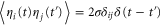
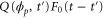
Let be the probability distribution function of the first passage time t' for the process represented by equation (1) from to with reflecting boundary at ; this condition applies to enzymes in a phase section, either or (with offset for the latter). Then,


where the rate corresponds to enzymes starting the cycle at and releasing a product at time t, i.e., after duration t'. Using Laplace transforms and of F and Q,


Similarly, for F1 in equation (3), the rate of the finish of the cycle is

and

Using the derivation in [18], the explicit form of for is


where . For (ideal delay),


The mean first passage time is


and the variance is
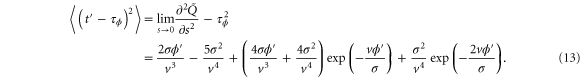
The mean cycle time τ is the sum of for the two sections before and after , i.e.,


Note that c, the total concentration of enzyme, is constant at each position x because the enzymes are not mobile; thus, from equations (2), (3), and (5), should be satisfied. In the present case, c is also spatially constant as the enzymes are uniformly distributed. The behavior of the system does not change if all of the concentrations are scaled with c, and if β is adjusted so that is kept unchanged: all the other parameters remain unaffected (note that in this model, only the binding of the product to the regulatory site is second-order, whereas the other reactions are first-order). In the stability analysis below, is adopted as a parameter.


We first consider concentrations , , and at the uniform steady state, satisfying


To attain this, the flux should be constant, i.e., from equation (5),

Using the mean cycle time τ, the total concentration of enzyme is represented by

Substituting equations (15)–(17) to equations (2)–(4), we obtain


where
(although there are two solutions, the other solution (substituting Z with in equations (18)–(20)) does not satisfy ).


This uniform steady state always exists. However, if it is unstable, small perturbations may grow into spatiotemporal patterns. To analyze the stability, we consider the deviations , , and from the steady state. We require the solutions for equations (2)–(4) in the following forms:


where q is the spatial wavenumber, and complex number λ corresponds to the growth rate and temporal (oscillation) frequency. Then, from equations (5) and (7),

so that

Similarly,

For small , , and around the steady state, equations (2)–(4) are linearized as:


with the linearization matrix

where and . Substituting equations (10), (14), (19), and (20) to equation (26), we obtain the explicit form of . Here, λ is one of the eigenvalues of , i.e., satisfying (see equations (21) and (25)), whereas contains and and, hence, depends on λ. Thus, has an infinite number of eigenvalues () that cannot be solved analytically. and represent the growth rate (i.e., the instability of the steady state) and frequency of the oscillatory mode, respectively. If is positive, the mode can grow when perturbation is applied to the steady state. We sort the modes in ascending order of fi. The 1st mode (f1) corresponds to the turnover frequency of each enzyme, and the ith mode () has a frequency approximately i times higher. Typically, (or slightly lower because the turnover time includes the waiting time between two consecutive cycles and, thus, is longer than the cycle time).


These discrete frequency modes (overtones) arise from the following mechanism. Let us consider a scenario with two groups of enzymes, as shown in figure 2. Each group of enzymes starts the cycle almost simultaneously, and the timing is shifted by approximately half a cycle between the groups. If , when one group arrives at and releases product molecules, the other group is approaching, or has just arrived at, ; thus, it can be efficiently activated by the product and start the next cycle. Consequently, such synchronized groups can be maintained, and the oscillations of concentrations are sustained. Although the turnover time of each enzyme cannot be shorter than the cycle time, the apparent oscillation period of the concentrations is halved, and this is the basis of the mode for which frequency is twice as high. Similarly, the ith mode corresponds to a scenario with i groups of enzymes in the phase space. We call this the i-group mode.


Figure 2. Mechanism of synchronization with multiple groups: case of the 2-group mode for . Suppose that there are two groups of enzymes with approximately half a cycle of phase difference. When one group releases product molecules, the other is approaching (or has just arrived at) the end of a cycle and can quickly be activated by the product and enter into the next cycle. Therefore, oscillations within these two groups may sustain their mutual activation of each other. The time series of concentrations shows frequency of oscillations that are twice as high as the turnover cycle for each enzyme ().


Download figure:
Standard image High-resolution imageAs predicted (and already reported for [7, 13]), the i-group mode is likely to grow if is close to a multiple of ; e.g., the 3-group mode may appear for or . Synchronization is also possible for close to 0, in which case a fraction of enzymes start the cycle spontaneously and soon release products, which in turn activate the remaining enzymes: this is typical in the 1-group mode. For , activation by products released by the same group of enzymes is possible, which also enables synchronization. The condition for synchronization is also affected by the diffusion of the product if we consider (spatial waves), as discussed in the section 3.


In the following sections, we solve the eigenvalue problem numerically and self-consistently by iteratively converging (Newton–Raphson method) from different initial values of λ, corresponding to different modes.
2.2. Stochastic simulations
When the density of enzymes is low, stochastic effects are not negligible. To consider such cases, we also adopted stochastic reaction–diffusion simulations. For simplicity, we assumed 1-dimensional space; in 2-dimensional space, target patterns, spiral waves, and wave turbulence appear [6, 7], but the basic properties discussed later are not affected.
The space is divided into Lx bins, and the enzymes are randomly distributed over the space and fixed. We set the volume of each bin to 1, there are and free enzyme molecules with and without regulatory products, and product molecules in the xth bin. The total number of enzyme molecules is . The product molecules diffuse, with the diffusion coefficient D [bin2/unit-time]. Additionally, a no-flux condition is applied. Binding of the product to the regulatory site of the enzyme in the same bin occurs at a rate of [/unit-time], and dissociation from the site occurs at [/unit-time]. We assume the substrate is abundant and its concentration is kept constant. Each free enzyme starts a cycle at rate (active enzyme) or (inactive enzyme) [/unit-time]. For each enzyme in the reaction cycle, the progress of the phase represented by equation (1) is simulated, with release of a product molecule at and return to the free state at . ϕ does not revert beyond the boundaries at and . Upon dissociation from the regulatory site and release from the catalytic site of the enzyme, the product molecule is placed in the same bin. Initially (t = 0), all the enzymes are free and no product exists.


Numerically, the progress of the enzyme phases and the diffusion of the product are processed at constant time intervals, whereas stochastic binding and dissociation at the regulatory site, initiation of a reaction cycle, and decay of the product are executed in each bin by the next reaction method [19].
3. Results
Unless otherwise stated, parameter values v = 1, , , , and were used in the analysis and simulations described below.


3.1. Intramolecular fluctuations
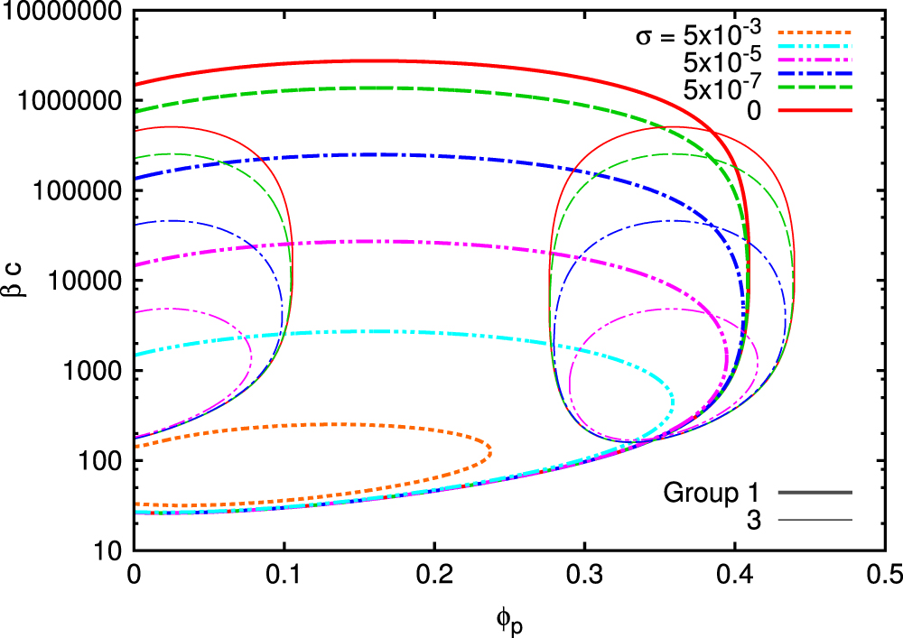
First, we show the uniform (well-mixed) case, which is similar to a previous study [14]. Bifurcation diagrams for the uniform case (zero wavenumber) for different strengths σ of intramolecular fluctuations are shown in figure 3. The upper boundary of β is drastically decreased by the intramolecular fluctuations, whereas the lower boundary is minimally affected. This is because if β is large, a small amount of the product released earlier via intramolecular fluctuations is sufficient to prematurely activate a significant proportion of free enzymes.

Figure 3. Bifurcation diagram for global synchronization (Hopf bifurcation). The thick line is for 1-group synchronization and the thin line is for 3-group synchronization. Colors show σ, the strength of intramolecular fluctuations.
Download figure:
Standard image High-resolution imageWhen we consider non-uniform cases, the growth rate of each mode also depends on the spatial wavenumber. In the current case, only the product can diffuse; therefore, the wavenumber q can be scaled by the diffusion coefficient D without loss of generality, resulting in the normalized wavenumber (see equation (26)). We calculated q' at which the growth rate takes the maximum value in (dominant wavenumber), as shown in figure 4 (the maximum growth rate and the frequency at the dominant wavenumber are also shown).


Figure 4. (a) Dominant wavenumber, i.e., the wavenumber at which the growth rate (real part of the eigenvalue) takes the maximum value; (b) maximum growth rate; and (c) frequency at the dominant wavenumber. . Only those wavenumbers and frequencies with a positive growth rate are plotted. The wavenumber is in the normalized form . For larger σ, the maximum growth rate is lower, whereas the dominant wavenumber and frequency are not significantly changed.


Download figure:
Standard image High-resolution imageFor some (e.g., 1-group mode with ), the dominant wavenumber is 0 and growth rate is positive, which means that global synchronization is strongest among the 1-group modes. For other cases, e.g., 1- and 3-group modes with , the dominant wavenumber is not zero (also see figure 5). Traveling or standing waves are expected to have a non-zero wavenumber.


Figure 5. (a) Growth rate for different numbers of groups plotted against normalized wavenumber . Cases with and are shown. , . (b) Schematic illustration of the dominant modes. 1- and 2-group cases in panel (a) are enlarged and shown with schematic pictures. The growth rate is maximal at a finite wavenumber for 1-group and at (i.e., global oscillation) for 2-group synchronization. The results of stochastic simulations with the same parameter values are shown in figure 6.


Download figure:
Standard image High-resolution imageAs previously reported [6, 7], wave bifurcation is possible even outside of the Hopf bifurcation (uniform oscillation) boundary shown in figure 3. In such cases, the growth rate is negative for but positive for a range of q'. When , the 1-group uniform mode vanishes at , whereas 1-group waves are possible up to with large wavenumbers (). For traveling waves, because the cycle time is almost constant, a larger wavenumber corresponds to slower propagation or to a longer delay from neighboring sites; thus, it is reasonable to suggest that such modes allow a communication delay through larger than uniform oscillations.


For larger σ, the maximum growth rate is lower, and synchronization is possible only in smaller parameter regions, as shown in figure 4(b); however, the dominant wavenumber and frequency do not change significantly (figures 4(a) and (c)).
Predictably, synchronization with many groups, i.e., at a high frequency, is sensitive to intramolecular fluctuations. If σ is large, only a small number of synchronized groups are allowed. However, 1-group synchronization is not always the most fluctuation-tolerant mode, especially in spatially non-uniform cases. For example, in the case shown in figure 5, the 2-group uniform (q = 0) oscillations are more robust against intramolecular fluctuations than the 1-group wave patterns with a finite wavenumber. Such an effect is indeed seen in numerical simulations; 2-group uniform oscillations are dominant in a certain range of σ, as shown in figure 6 (center column).

Figure 6. Spatiotemporal patterns for different concentrations of enzymes c and intramolecular fluctuations σ. and =104. The color shows product concentration p: black for p = 0 to white for . The horizontal axis corresponds to the spatial position (1-dimensional). [bins] and D = 1000 [bin2/unit-time]. Time is displayed from the top to the bottom in each panel. In order to show the transient behavior, data for and are displayed. Standing waves with one synchronized group are sensitive to intramolecular fluctuations; hence, 2-group global oscillations are dominant when σ is large (center column). In contrast, with a low density of enzymes (right column), 1-group standing waves are enhanced. These data can be compared with the schematic representations in figure 5 (b) (also see supplementary movies 1 and 2 available at stacks.iop.org/njp/17/033024/mmedia).


Download figure:
Standard image High-resolution image3.2. Intermolecular fluctuations
We have considered fluctuations that originate from the internal states of the enzymes; however, there is another potential source of fluctuations: the stochastic binding, dissociation, and decay of molecules. In a biological cell, the concentration of an enzyme species is not always high. If molecular events such as collision, binding, and release involve a low concentration of enzymes, they are inevitably stochastic and show large fluctuations in their rate.
Because we can change the enzyme concentration c without affecting the behavior in the continuum limit if is kept unchanged, we can investigate the effects of stochasticity. In figures 6 and 7, spatiotemporal patterns for two different enzyme concentrations are shown. At a low concentration, synchronization between the enzymes is more stochastic and often disturbed. Of course, at a concentration much lower than one enzyme per the diffusion length of the product (i.e., the distance the product diffuses before decaying), enzymes can no longer communicate and synchronization is lost. However, such stochasticity (variation in the waiting time) may even strengthen certain synchronization modes, in contrast to the intramolecular fluctuations (variation in the cycle time), which merely hinder synchronization.


Figure 7. Spatiotemporal patterns for different concentrations of enzymes c and intramolecular fluctuations σ, with . = 104, and D = 1000. Notations are the same as in figure 6. With a low density of enzymes (right column), i.e., larger intermolecular fluctuations, synchronization modes with 5 groups rapidly grow. In contrast, intramolecular fluctuations suppress the growth of such high frequency modes; hence, 1- and 3-group synchronization is more dominant in the left bottom panel.


Download figure:
Standard image High-resolution imageIn some parameter regions, two or more modes (frequencies) are possible. With such parameters, stochastic fluctuations affect the selection of modes: an example is shown in figure 7. In this case, the parameters allow mixed modes. Where the concentration of enzymes is high (see left panel in figure 7), synchronization with 1 group occurs first, while it grows very slowly with 3 or 5 groups. In contrast, at a low enzyme concentration (right panel in figure 7), synchronization with 3 or 5 groups is induced much more quickly by the stochastic noise. This behavior is similar to noise-enhanced phase synchronization [20]; however, the frequency depends on the intrinsic dynamics of the enzymes.
It is also important to understand whether synchronization waves can be induced in a system where synchronization is not observed without fluctuations. Near the boundary of parameters for synchronization, once the enzymes are synchronized, oscillatory patterns may sustain for some cycles. If fluctuations are present, weakly oscillating patterns may appear. On some occasions, complete synchronization can almost be recovered even if β is so high that synchronization is impossible in the continuum limit. For this type of synchronization, the discreteness of the enzymes plays an important role.
In the continuum limit, the concentrations can be infinitesimally small but non-zero. Even in synchronized states, there is always a small fraction of free enzymes that can start a cycle. Although the decay of the product is fast, a small fraction of the regulatory product may remain after cycling and activate the enzymes asynchronously. If β is too high, this residual product can gradually desynchronize the enzymes. However, with discrete molecules, the numbers of the product and free enzyme molecules should be integers and reach 0 at some point, thereby hindering such step-by-step desynchronization and sustaining the synchronized state.
The situation in this stochastic synchronization is analogous to discreteness-induced transitions, previously reported by one of the authors [10, 21]. No matter how fast the positive feedback reaction progresses, it completely stalls when the relevant molecules vanish. In the previously reported case [10, 21], for the transitions to occur, decay of a certain chemical species had to be faster than the interval of molecular inflow of the chemical; however, in the present case, decay must be sufficiently faster than the turnover time, although the threshold is also affected by β.
3.3. Fluctuation-dependent mode selection
Intramolecular fluctuations decrease the upper limit of β for synchronization in the continuum limit, as shown in figure 3. In contrast, intermolecular fluctuations may induce synchronization even if β is larger than the limit, i.e., they increase the effective upper limit of β. For synchronization with 2 or more groups, these effects are significant. In spatially distributed cases, the boundary of and β for synchronization also depends on the wavelength. Hence, the combination of intra- and intermolecular fluctuations may determine the synchronization mode (frequency and wavelength) that appears.

Figure 6 shows an example of such effects observed in stochastic simulations. Without any fluctuations, 1-group standing-wave patterns and 2-group global synchronization are possible (figure 5), although the parameter values are close to the bifurcation boundary. Mixed behavior is indeed observed with and c = 1000 (figure 6, left column). The 1-group standing-wave patterns are enhanced under stronger intermolecular fluctuations (c = 10 with fixed; right column), whereas the 2-group global synchronization dominates under moderate intramolecular fluctuations (; center column).


4. Discussion
As indicated in this study, the two sources of fluctuations may work distinctively and complementarily, although both have only been regarded as 'fluctuations' in the general context of biochemical systems.
When interpreting the behavior of the model for actual biological systems, the relationship between the parameters is important. Among the kinetic parameters, we focused on β as it directly controls the binding to the regulatory site of the enzyme. However, in addition, and γ must be sufficiently high compared with the cycle time in order to ensure regulation is fast enough for synchronization. It enforces the lower limit of γ at .


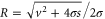
The spatiotemporal phenomena discussed here depend on communication between the enzymes via the product; hence, the diffusion of the product plays a key role. The diffusion length of the product is . Unless the neighboring enzymes are within this distance, they cannot communicate. If the product should find its target (regulatory site) by free normal diffusion in three dimensional space, the mean time to find a target is approximately , where L is the typical distance between targets (assuming the targets are uniformly distributed) and R is the radius of the target [6, 13]. For a product to find a target within its lifetime, , i.e., is required. As is often observed in the cell, if the searching process involves subdiffusion and D represents the macroscopic diffusion coefficient, the limit may be less stringent, but still cannot exceed ldiff.


Due to the lower limit of γ, if the cycle time occurs in around 1 s, γ should be at least ∼1 s−1. D may vary in the cell; for example, it can range from 10−3 μm2 s−1 for macromolecules embedded in the membrane or in a crowded environment to 103 μm2 s−1 for free small molecules. The corresponding upper limit of the distance between enzymes by the former condition (ldiff) is tens of nanometers to tens of micrometers, whereas by the latter condition (transit time) it is 10 nm–1 μm, assuming nm. As L = 1 μm roughly corresponds to 1 nM, it is a plausible value for the actual physiological concentrations of enzymes. Near the limit, the communication becomes stochastic, leading to strong intermolecular fluctuations.

In the case considered here, the normalized wavenumber q' reached only ∼1. This can be considered natural because patterns that are finer than the diffusion length ldiff of the product cannot be sustained against spatial averaging by diffusion (wavelength corresponds to ). Hence, in order to observe spatial patterns, ldiff should be much smaller than the size of the system (e.g., the cell). It is possible that, given the estimation above, μm holds for the product lifetime milliseconds to minutes.


Although we showed only one-dimensional examples in figures 6 and 7, the synchronization mechanism should also work in two or three dimensional systems, and the stability analysis adopted here should also be valid. Simulation examples of two dimensional cases are shown in supplementary movies 1 and 2.
In actual biochemical reactions, intramolecular fluctuations cannot be very small for a single enzyme. However, if a certain set of reactions must occur consecutively, the standard deviation of the total elapsed time for the reactions can be significantly smaller than the average, even if each reaction involves large intramolecular fluctuations. Gruler et al experimentally demonstrated the long cycle time (1.54 s) of the cytochrome P-450 mono-oxygenase system [5] and suggested a model for the reaction cycle that included many substeps [22]. In the cell, membrane compartments and scaffold proteins may also facilitate a chain of reactions. Fast oscillatory patterns observed in the cell (e.g. [23], although still controversial) may depend on the intrinsic cycle time of such a molecular system. Our analytical scheme is also applicable to reaction chains at longer timescales, where compensation mechanisms for the delay may also exist [24]. Theoretically, intramolecular fluctuations of a different nature can be considered by the same analytical scheme as long as the transfer functions rp and r can be obtained.
There are a wide variety of molecules in the cell; thus, some chemical species must inevitably be rare. This has often been discussed in the context of stochastic gene expression [25]; however, it applies not only to DNA and mRNA but also to proteins. Recently, in bacterial cells, many protein species were shown to exist at very low levels of molecule/cell [26], i.e., sometimes they existed in the cell, and sometimes they did not. If such a chemical is involved in the reaction network, the behavior of the system becomes stochastic, i.e., it shows strong intermolecular fluctuations, and the state or individuality (dynamic disorder [27, 28]) of each molecule may significantly affect the system. The intensity of intermolecular fluctuations may also depend on the effective system size. Cells are crowded with macromolecules; for example, while eukaryotic cells are large, they include complex structures such as membrane compartments and cytoskeletal components, and these can limit the effective volume of the system and the number of molecules that can join reactions.

The processes in the cell require a balance of the two types of fluctuations studied here. Therefore, their effects should be considered further in the context of complex reaction networks in the cell. Although our current model deals only with a single enzyme species and a straightforward reaction process, it could be extended to multiple reaction paths [15] and combined into a network. Moreover, at macroscopic levels, similar effects may appear if delayed feedback mechanisms and fluctuations exist, e.g., gene expression delays in morphogenesis [29], or circadian clocks. We suggest that our simplified model and analysis may provide a convenient way to model such a network involving delays and fluctuations.
Acknowledgments
We thank Alexander S Mikhailov, Masahiro Ueda, Tatsuo Shibata, and Hiroaki Takagi for helpful comments. This work was supported by the Ministry of Education, Culture, Sports, Science, and Technology, Japan (KAKENHI 20740243 and 23115007 'Spying minority in biological phenomena', and Platform for Dynamic Approaches to Living System) and the Japan Society for the Promotion of Science. The large-scale computing system of the Cybermedia Center, Osaka University was used for part of the study.